A depth camera on an industrial arm can produce hundreds of thousands of points from one view. Many samples describe almost the same patch of a table or component. Feeding every sample into registration or clustering costs time without adding the same amount of useful geometry.
Dense input
Downsampled output
1. What is Voxel Downsampling?
Voxel downsampling divides 3D space into equal cubes and replaces all points inside each occupied cube with one representative point. This tutorial explains how points are assigned to voxels, why the representative is usually a centroid, and how voxel size becomes both a compute budget and a geometric resolution limit.
A voxel is the three-dimensional equivalent of a pixel. A pixel covers an area on a 2D image grid; a voxel covers a volume on a 3D grid. The grid is not trying to recognize objects. It is a bookkeeping structure that asks which samples occupy approximately the same region of space.
This makes voxel downsampling different from taking every tenth row of a point array. Array order may follow camera scan order and says little about spatial redundancy. Voxel filtering responds to geometry: a densely sampled surface loses more points than a sparse region because more samples fall into the same cells.
1.1 The Complete Voxel-Grid Pipeline
Dense samples → one representative per occupied cell
Voxel size is both a speed control and a geometric resolution limit: features smaller than a cell can disappear.
The pipeline starts with a dense point cloud and one engineering choice: the edge length of a cubic voxel. That length is expressed in the cloud’s coordinate units. A value of 0.005 means five millimetres only when the cloud uses metres.
The grid gives every point a discrete cell address. Points with the same address are grouped. Each non-empty group is then summarized by its centroid, producing one output position for the occupied voxel. Empty cells produce no point, so the result remains a point cloud rather than a dense 3D image.
The output follows the broad shape of the input with fewer, more evenly spaced samples. Increasing voxel size accelerates later operations but progressively removes narrow gaps, thin edges, and small features. The remainder of the tutorial makes that trade-off measurable.
1.2 How a Point Gets a Voxel Address
Let the voxel edge length be and let the grid origin be . A point receives integer voxel index
is the three-integer cell address; division and floor are applied component by component; is the voxel size; and rounds toward negative infinity. Any points that produce the same belong to the same voxel.
The exact origin shifts cell boundaries, but it does not change the basic resolution. A point that lies very close to a boundary can move to a neighboring cell under small sensor noise. This is usually acceptable for downsampling, but it explains why the result is not invariant to an arbitrary grid translation.
1.3 Why the Output Point Is the Centroid
For occupied voxel , let be the indices of its input points. The representative is
is the output centroid, is the number of samples in voxel , and is the set of samples assigned to that cell. Unlike using the cell center, the centroid responds to where the measured surface actually passes through the cube.
The centroid minimizes the sum of squared distances to the points in that voxel. It may not be one of the original sensor samples, and it may lie slightly away from a curved surface when a large voxel spans that curve. This is one reason voxel size must stay below the scale of geometry that matters.
Interactive voxel grid
Increase cell size and watch nearby samples share one representative
Colors and normals can also be aggregated when they are present. Averaging colors is usually intuitive. Averaging normals requires normalization afterward and can become misleading if one voxel straddles a sharp corner whose surfaces point in different directions.
1.4 Voxel Size Controls Resolution and Work
Suppose two parallel surfaces are separated by distance . If is comparable to or larger than , samples from both surfaces may enter the same voxel and collapse into a representative between them. A graspable gap can disappear even though the overall object still looks recognizable.
At the other extreme, a voxel smaller than the sensor’s point spacing changes little. Most occupied cells contain only one point, so the algorithm adds grid construction without reducing later work.
A practical starting point is two to five times the typical point spacing, then adjust according to the smallest feature that must survive. The Telekinesis documentation suggests choosing a cell slightly larger than sensor noise but smaller than the smallest required detail. These are not universal numbers: a drone mapping a wall and a cobot inspecting a connector have very different spatial scales.
The maximum possible geometric displacement introduced by a representative depends on the samples inside a cube. The cube diagonal is
is the corner-to-corner voxel distance and is its edge length. This does not say the centroid error will equal the diagonal, but it gives a useful scale for judging whether a cell is grossly larger than the task tolerance.
1.5 Why Density Becomes More Uniform
Depth sensors often sample surfaces unevenly. Nearby regions occupy more pixels and can contain many more points than distant regions. Reflective or grazing surfaces may be sparse. If registration minimizes an unweighted sum over all samples, dense regions can dominate the solution simply because they contribute more terms.
Voxel downsampling caps this influence at roughly one representative per occupied spatial cell. The density does not become perfectly uniform—surface orientation and occlusion still matter—but the disparity is reduced. That often makes neighbor searches, normal estimation, ICP, and feature computation faster and better conditioned.
Uniform index downsampling cannot make the same guarantee. If a block of 1,000 consecutive array entries covers one tiny surface patch, selecting every tenth entry still gives that patch 100 samples.
1.6 Where It Belongs in a Robotics Pipeline
For an AMR building a local map, downsampling can keep successive scans manageable before registration. For a cobot, it can simplify the scanned surface of a large casting before pose refinement. For a humanoid, it can reduce the ground and furniture geometry used in short-horizon planning. For a drone, it can control map growth while retaining the structures needed for localization.
A common ordering is:
raw cloud
→ crop to the relevant workspace
→ remove obvious outliers
→ voxel downsample
→ estimate normals or descriptors
→ cluster, register, or reconstruct
Cropping first avoids spending voxel cells on irrelevant space. Estimating normals after downsampling ensures the normals belong to the geometry the next algorithm will actually use. There are exceptions—fine normal estimation may require the original cloud—but the order should be chosen deliberately.
1.7 Failure Modes and Artifacts
Large voxels round sharp corners, bridge narrow gaps, and remove thin objects. A wire, sheet edge, or gripper finger can disappear even while a large housing remains clear. Always inspect the smallest task-relevant feature, not only the overall silhouette.
The filter also does not remove isolated outliers by definition. A lone noise point in its own voxel still creates one output point. Radius or statistical outlier removal solves a different problem.
Finally, downsampling is lossy. Keep the original cloud when later metrology or final surface fitting needs full resolution. A useful design is coarse-to-fine: use a downsampled cloud to estimate a pose quickly, then evaluate or refine that pose against the original samples.
1.8 A Worked Registration Example
Consider a cobot that scans a machined housing from two viewpoints. Each raw scan contains 600,000 points. The smallest chamfer used for alignment is 8 mm wide, the median neighbor spacing on the housing is about 1.5 mm, and random depth variation is close to 1 mm.
A 1 mm voxel is unlikely to help: it is no larger than the noise and many cells still contain one sample. A 20 mm voxel would be fast, but it can erase the 8 mm chamfer. Testing 3, 5, and 7 mm gives a more useful experiment. Suppose 5 mm reduces each cloud to 85,000 points while preserving the chamfer and maintaining registration accuracy. That becomes the coarse alignment representation.
The final pose need not remain limited to 5 mm geometry. After coarse alignment and ICP on the downsampled clouds, the cobot can transform the original scan and perform a final narrow-distance refinement against full-resolution samples. The grid bought speed where broad shape was enough without discarding precision from the final measurement.
This experiment should be repeated when camera resolution, working distance, or object family changes. Voxel size is a physical length, but the number of raw samples inside that length depends on all three.
1.9 Voxel Grids Are Not Occupancy Maps
Both concepts divide space into cells, but their outputs serve different purposes. Voxel downsampling emits one representative point for each cell that received samples. It does not normally label unseen cells as free or occupied, estimate visibility, or accumulate probabilistic evidence over time.
An occupancy map reasons about free, occupied, and sometimes unknown space, often by tracing sensor rays. It supports navigation and collision checking. A downsampled cloud is a lighter geometric sample set for algorithms such as registration, clustering, and surface processing.
The distinction prevents a dangerous inference: absence of a point in the downsampled output does not prove that space is free. It may be occluded, outside the sensor view, reflective, or simply empty at the chosen sampling resolution.
Keep that distinction explicit in interfaces: name the output downsampled_cloud, not occupancy_grid, and never send it directly to a collision checker that expects observed free space. A geometric simplification preserves samples; it does not create a visibility model.
2. Using Voxel Downsampling in the Telekinesis Agentic OS
Telekinesis provides filter_point_cloud_using_voxel_downsampling as a Vitreous Skill:
from telekinesis import datatypes, vitreous

point_cloud = datatypes.PointCloud.from_url(
    url=(
        "https://assets.telekinesis.ai/examples/v1/point_clouds/"
        "can_vertical_1_subtracted.ply"
    ),
    use_cache=True,
)

downsampled = vitreous.filter_point_cloud_using_voxel_downsampling(
    point_cloud=point_cloud,
    voxel_size=0.005,
)

print("input points:", len(point_cloud))
print("output points:", len(downsampled))
print("reduction:", 1 - len(downsampled) / len(point_cloud))
The result is a datatypes.PointCloud with one centroid per occupied voxel. The Skill preserves normals and colors when the input contains them. voxel_size must be greater than zero and uses the cloud’s coordinate units.
3. How to Benchmark a Voxel Size
For several candidate sizes, record output point count, processing time, downstream latency, and task error. For registration, compare final pose error and convergence rate. For clustering, compare object splits and merges. For grasping, check whether contact surfaces and openings survive.
Do not choose the largest reduction that still “looks fine” in a viewer. Rendered points have screen-space size and can hide missing geometry. Measure surface distance against the original cloud and evaluate the actual downstream task.
4. Where to Go Next
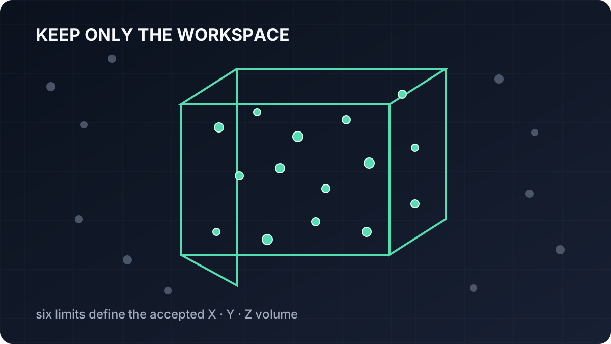 Basic · 11 min read
What is a Pass-Through Filter?
A pass-through filter removes 3D points outside a known workspace by applying minimum and maximum limits along X, Y, and Z. Learn how the crop works, why coordinate frames and units matter, how to tune its six bounds, and how to use it in the Telekinesis Agentic OS.
Read tutorial →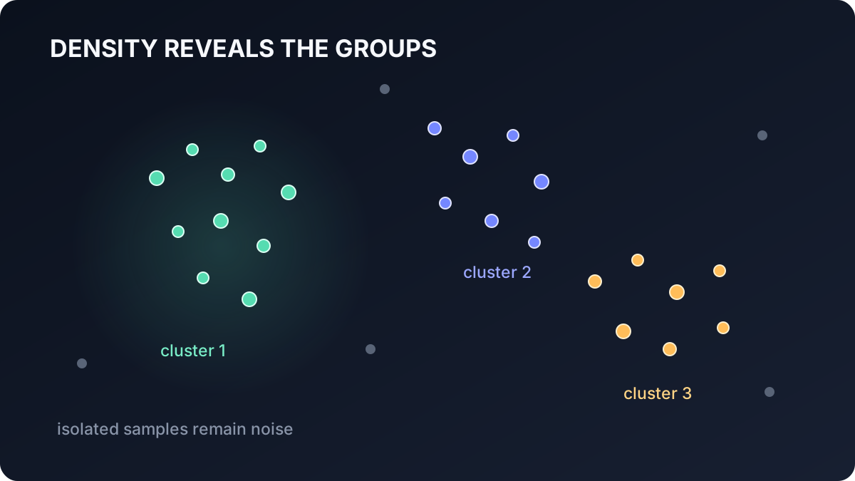 Intermediate · 10 min read
What is DBSCAN Point-Cloud Clustering?
DBSCAN separates a point cloud into dense connected groups without requiring the number of clusters in advance. Learn core, border, and noise points, density reachability, parameter tuning, computational trade-offs, and how to use DBSCAN in the Telekinesis Agentic OS.
Read tutorial →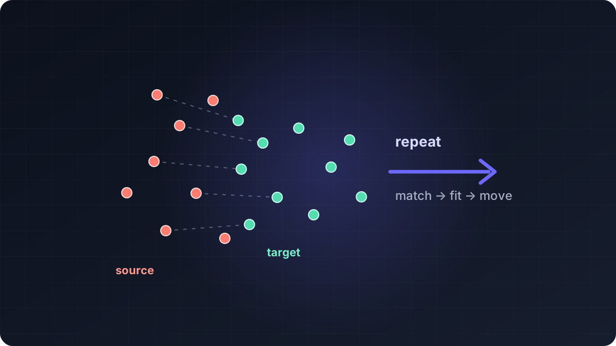 Advanced · 17 min read
What is Iterative Closest Point (ICP)?
Point-cloud registration solves the problem of placing two 3D scans in the same coordinate frame, and ICP does this by repeatedly matching nearby points and fitting a rigid transform. Learn point-to-point and point-to-plane ICP, Fast Global Registration, their mathematics and failure modes, and how to build a coarse-to-fine registration pipeline in the Telekinesis Agentic OS.
Read tutorial →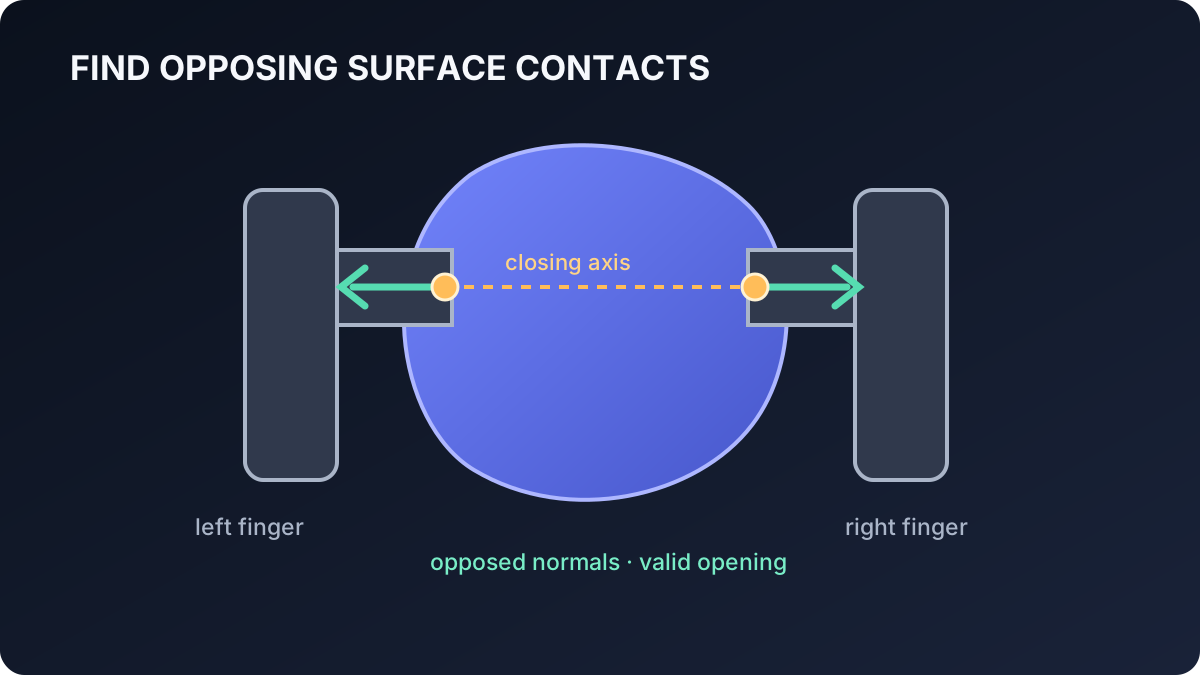 Advanced · 11 min read
What is Antipodal Grasp Sampling?
Antipodal grasp sampling proposes parallel-jaw grasps by finding opposing contacts on an object surface. Learn contact normals, friction intuition, grasp-frame construction, candidate scoring and validation, and how to generate grasps in the Telekinesis Agentic OS.
Read tutorial →5. References
- Telekinesis. “Filter Point Cloud Using Voxel Downsampling”, Vitreous Skill documentation.