Imagine an industrial arm looking into a tote after the floor and walls have been removed from its depth scan. Several components remain as disconnected islands of 3D points. The robot needs to turn that one point cloud into separate candidate objects, but it does not know in advance whether the tote contains two parts or twelve.
Combined point cloud
Calculated clusters
1. What is DBSCAN Point-Cloud Clustering?
DBSCAN groups nearby points into dense connected regions and labels points outside those regions as noise. In this tutorial, you will learn what “dense” means mathematically, how clusters grow from core points, why two parameters control both object separation and noise rejection, and where the result can mislead a robot.
DBSCAN stands for Density-Based Spatial Clustering of Applications with Noise. Unlike k-means, it does not require an engineer to specify the number of clusters. It can also recover curved or irregular groups rather than forcing every cluster to look roughly spherical around a center.
That makes it useful for point clouds, where one object may form an uneven shell and isolated depth errors should not become objects of their own. But DBSCAN knows nothing about object identity. If two parts touch through a dense bridge of samples, it may merge them. If one part contains a large density change, it may split it.
1.1 The Complete DBSCAN Pipeline
Local point density → clusters and noise
DBSCAN discovers how many groups exist, but “dense and connected” is a geometric rule—not proof that every group is one object.
The algorithm begins with a point cloud and two definitions of density. The first, usually called epsilon or , is the radius of a local neighborhood. The second, min_points, says how many samples must occupy that neighborhood before its center counts as a dense core point.
DBSCAN examines local neighborhoods and finds those cores. It then connects core points whose neighborhoods overlap. Each connected dense region grows into a cluster, and nearby non-core samples can join as border points. Samples that cannot reach any dense region remain noise.
The output is therefore not produced by choosing a cluster count. It emerges from a physical scale and a sampling-density rule. Understanding those two choices is the key to using DBSCAN rather than merely calling it.
1.2 The Epsilon Neighborhood
For point , its closed epsilon neighborhood is
is the set of samples within radius of point ; is another 3D sample; and is Euclidean distance. The neighborhood normally includes itself, so confirm the convention when comparing implementations.
is expressed in the point cloud’s units. If the cloud uses metres, 0.01 is a one-centimetre radius. That number should relate to point spacing and the smallest physical gap meant to separate objects.
1.3 Core, Border, and Noise Points
A sample is a core point when
where is set size and is min_points. Core points have enough local support to begin or expand a cluster.
A border point has fewer than neighbors but lies inside the epsilon neighborhood of a core point. It can join that core’s cluster but cannot independently expand the cluster. A noise point is neither a core nor reachable as a border point when clustering finishes.
These labels depend on the selected parameters. “Noise” does not necessarily mean a bad sensor sample. A small but real fastener may be too sparse to meet the density rule.
Interactive density clustering
Change ε and min_points to see clusters grow, split, or become noise
1.4 How Density Reachability Grows a Cluster
Suppose point lies within of core point . Then is directly density-reachable from . If is also a core, its neighborhood can extend the region further. Repeating this connection produces a chain of dense neighborhoods.
This chaining is why DBSCAN can follow a curved cable or irregular casting. No centroid dictates the shape. It is also why a narrow but sufficiently dense bridge between two objects can merge them into one cluster.
A simplified algorithm is:
mark every point unvisited

for each unvisited point p:
    find neighbors within epsilon
    if neighbor count < min_points:
        mark p as noise for now
    else:
        start a new cluster
        add p and repeatedly visit its neighbors
        whenever a visited neighbor is also a core point,
        add its neighborhood to the expansion queue
A sample marked noise early can later become a border point when reached from a core. The label is provisional until all dense regions have been expanded.
1.5 Choosing Epsilon from Point Spacing and Object Gaps
The radius must be large enough to connect samples on the same physical surface, including sparse areas. It must stay smaller than gaps that should separate objects. Those requirements can conflict.
A useful diagnostic is the k-distance plot. Choose related to min_points, compute each sample’s distance to its th nearest neighbor, sort those distances, and look for an elbow where sparse regions begin. That elbow can suggest an epsilon value, but it is not an automatic truth—mixed-density clouds may have several scales and no clean elbow.
Sensor geometry matters. A depth camera often samples nearby surfaces more densely than distant ones. One global may merge nearby objects yet fragment distant ones. Cropping by range, voxel downsampling to more even spacing, or clustering separate depth bands can make the density assumption more realistic.
1.6 Choosing min_points
Low min_points admits small clusters but also makes random clumps easier to accept. A higher value demands stronger evidence and rejects more isolated samples, but can erase small or sparsely observed objects.
In three dimensions, a common conceptual starting point is at least four points, but there is no universal best value. The appropriate count depends on voxel size, surface sampling, occlusion, and the minimum object size. Telekinesis documents a typical exploratory range of roughly 3–50.
The two parameters cannot be tuned independently. Increasing increases neighborhood counts, so the same min_points becomes easier to satisfy. Always evaluate the pair together.
1.7 Why Preprocessing Changes the Answer
A pass-through crop removes walls, robot geometry, and remote surfaces that could form dominant clusters. Voxel downsampling reduces density variation and makes a distance parameter easier to interpret. Plane removal prevents the table from connecting every object that touches it.
This is not cosmetic preprocessing. DBSCAN’s definition of a cluster is based entirely on distances and counts, so any operation that changes spacing or removes samples changes the cluster topology. Record the preprocessing configuration together with and min_points.
1.8 Computational Cost
A naive implementation compares every pair of points and costs distance checks for samples. Spatial indexes such as k-d trees or voxel hashes reduce neighborhood-query cost in ordinary cases, often toward overall, though exact behavior depends on dimension, distribution, and implementation.
This explains a practical pipeline: crop first, downsample second, cluster third. Reducing the cloud from 500,000 to 50,000 relevant samples can matter more than a small code-level optimization.
1.9 Robotics Failure Modes
Touching components can merge. One component with sparse reflective surfaces can split. A human hand entering the crop can form a perfectly valid cluster. Dense sensor artifacts can become false clusters, while a thin real object can be labeled noise.
Treat each cluster as a geometric proposal. Validate it with size, bounding-box dimensions, color, learned classification, CAD registration, or task-specific constraints. For grasping, also check that the cluster contains enough complete surface geometry to plan contacts.
1.10 A Worked Tote Example
Suppose a cobot observes metal components in a tote with millimetre-scale point-cloud coordinates. After plane removal and 4 mm voxel downsampling, neighboring points on one component are usually 4–7 mm apart. Separate components should have at least 25 mm of free space between them.
An engineer begins with max_distance=10 mm and min_points=6. The radius connects ordinary surface samples without jumping the expected object gap. On validation scenes, thin tabs at the back of the tote are sparser and become noise, so epsilon is raised to 13 mm. That recovers the tabs, but two parts separated by a narrow 20 mm gap begin to merge.
This is not a parameter-tuning accident; the requirements overlap. One global radius cannot both bridge a 13 mm sampling gap and guarantee separation across every 20 mm object gap when chains of intermediate points exist. Options include improving the scan, using a smaller voxel, removing contact bridges using surface normals, splitting a merged cluster later, or adding image-instance masks.
The worked example illustrates the correct lesson from a failed sweep: sometimes the representation violates DBSCAN’s density assumptions. More searching over the same two parameters cannot create missing geometric evidence.
1.11 DBSCAN Compared with Nearby Alternatives
Euclidean connected-component clustering links samples that fall within a distance threshold and is close to DBSCAN with a very permissive density requirement. It preserves tiny groups but is more likely to promote noise into objects. K-means requests a fixed number of clusters and assigns every point, which is inconvenient when object count changes and noise should remain unassigned.
Plane segmentation solves another problem: it finds a dominant surface model such as a floor, wall, or table. Removing that plane often makes DBSCAN more effective, because otherwise the shared support surface can connect all resting objects.
Learned 3D instance segmentation can use shape and semantics to separate touching objects, but it introduces training data, inference cost, and domain-shift concerns. DBSCAN remains valuable when spatial separation is the main signal and its assumptions match the workcell.
1.12 Making Cluster IDs Safe to Use
Cluster indices are usually arbitrary results of one invocation. Cluster 0 in the current cloud is not automatically the same physical object as cluster 0 in the next frame. An AMR or humanoid that needs persistent identities must add tracking based on position, appearance, shape, or motion.
Before acting, calculate simple cluster properties: point count, centroid, axis-aligned or oriented bounds, distance from the camera, and proximity to workspace boundaries. Reject physically impossible sizes and flag clusters cut by the crop. These checks are inexpensive and make failure behavior visible before a planner commits to a target.
2. Using DBSCAN in the Telekinesis Agentic OS
Telekinesis provides cluster_point_cloud_using_dbscan through Vitreous:
from telekinesis import datatypes, vitreous

point_cloud = datatypes.PointCloud.from_url(
    url="https://assets.telekinesis.ai/examples/v1/point_clouds/mounts_3_raw.ply",
    use_cache=True,
)

cropped = vitreous.filter_point_cloud_using_pass_through_filter(
    point_cloud=point_cloud,
    x_min=-185.0,
    x_max=230.0,
    y_min=-164.0,
    y_max=164.0,
    z_min=450.0,
    z_max=548.0,
)

clusters = vitreous.cluster_point_cloud_using_dbscan(
    point_cloud=cropped,
    max_distance=8.0,
    min_points=10,
)

print("clusters:", len(clusters))
for index, cluster in enumerate(clusters):
    print(index, len(cluster), cluster.positions.min(axis=0), cluster.positions.max(axis=0))
max_distance is the DBSCAN epsilon and uses the cloud’s coordinate units. The example values fit this millimetre-scale asset; retune them for another sensor and preprocessing chain.
3. How to Evaluate Clustering
If object-level labels exist, measure over-segmentation, under-segmentation, missed objects, false clusters, and cluster purity. Also evaluate the downstream task: can each cluster be registered, classified, or grasped correctly?
Create scenes with varying object separation, partial contact, range, surface reflectivity, and occlusion. Include the smallest supported object and the largest expected density change. Report the complete preprocessing and units so the parameters remain meaningful.
4. Where to Go Next
 Basic · 11 min read
What is a Pass-Through Filter?
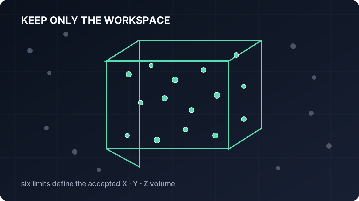
A pass-through filter removes 3D points outside a known workspace by applying minimum and maximum limits along X, Y, and Z. Learn how the crop works, why coordinate frames and units matter, how to tune its six bounds, and how to use it in the Telekinesis Agentic OS.
Read tutorial →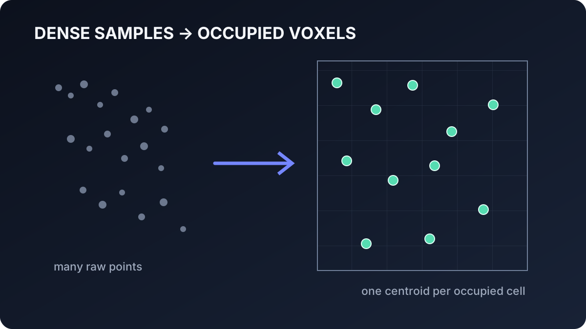 Basic · 10 min read
What is Voxel Downsampling?
Voxel downsampling reduces a dense point cloud by replacing samples in each occupied 3D cell with their centroid. Learn how voxel indexing and averaging work, how voxel size trades geometric detail for speed, and how to use the filter in the Telekinesis Agentic OS.
Read tutorial →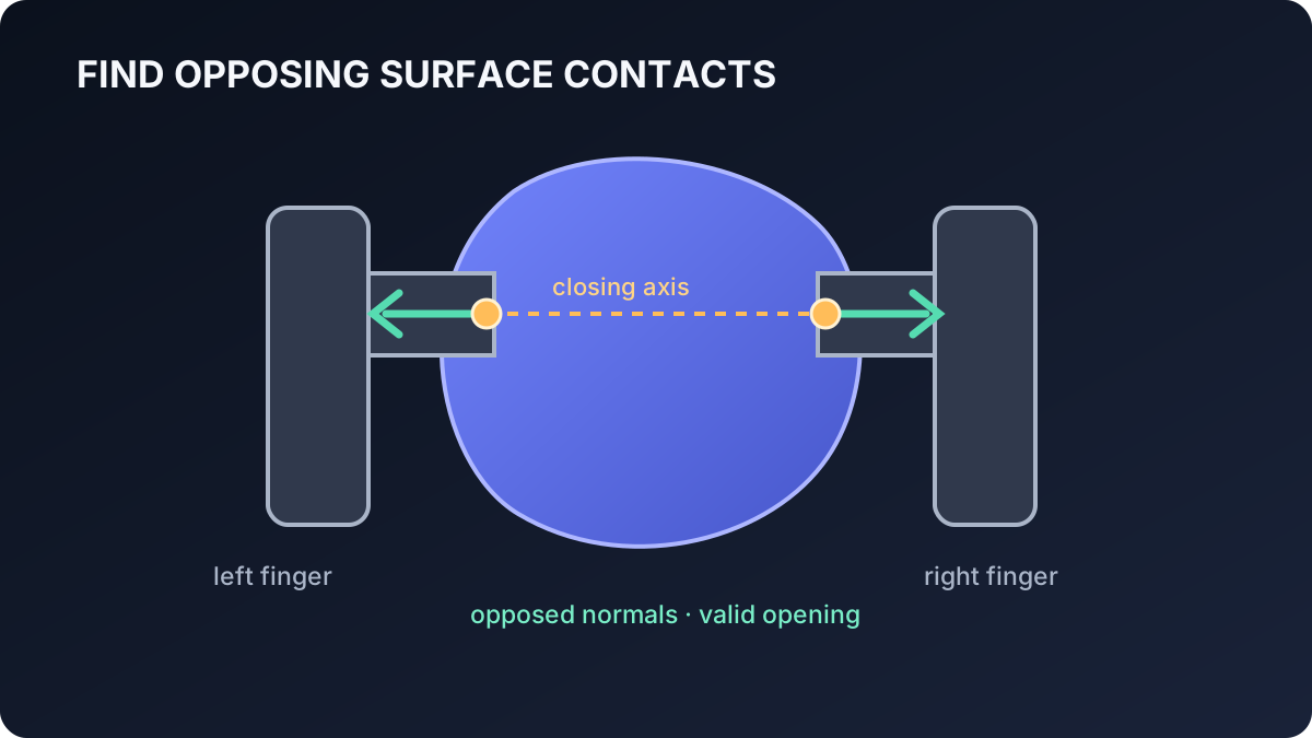 Advanced · 11 min read
What is Antipodal Grasp Sampling?
Antipodal grasp sampling proposes parallel-jaw grasps by finding opposing contacts on an object surface. Learn contact normals, friction intuition, grasp-frame construction, candidate scoring and validation, and how to generate grasps in the Telekinesis Agentic OS.
Read tutorial →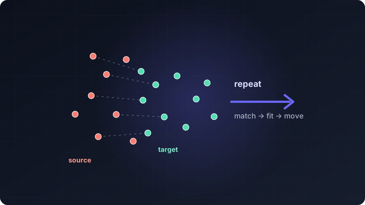 Advanced · 17 min read
What is Iterative Closest Point (ICP)?
Point-cloud registration solves the problem of placing two 3D scans in the same coordinate frame, and ICP does this by repeatedly matching nearby points and fitting a rigid transform. Learn point-to-point and point-to-plane ICP, Fast Global Registration, their mathematics and failure modes, and how to build a coarse-to-fine registration pipeline in the Telekinesis Agentic OS.
Read tutorial →5. References
- Ester, M. et al. “A Density-Based Algorithm for Discovering Clusters in Large Spatial Databases with Noise”, KDD, 1996.
- Telekinesis. “Cluster Point Cloud Using DBSCAN”, Vitreous Skill documentation.