Imagine a cobot looking into a parts tray with a depth camera. The scan contains the parts, but it may also contain the table, a safety fence, the camera stand, and points behind the workcell. The robot does not need a clever model to reject most of that geometry. It already knows where the tray is.
Raw point cloud
Filtered points
1. What is a Pass-Through Filter?
A pass-through filter keeps point-cloud samples inside a chosen three-dimensional box and removes the rest. In this tutorial, you will learn how six coordinate limits define that box, why the cloud’s frame and units matter more than the comparison itself, and where this simple operation belongs in a robot perception pipeline.
The core idea is to use knowledge that the robot already has. If an industrial arm only handles parts between 45 and 55 centimetres above its base, points near the ceiling cannot describe a grasp target. If an AMR is checking a shelf on its right, points behind the sensor are irrelevant to that task. Removing those regions early reduces data transfer and gives clustering, registration, or pose estimation less distracting geometry to process.
This is a geometric filter, not an object detector. It cannot tell a component from a human hand when both occupy the accepted volume. It answers a narrower question: is this sample inside the region we chose to inspect?
1.1 The Complete Filtering Pipeline
3D workspace bounds → relevant points
The filter does not recognize objects; it removes space that the robot has already decided cannot matter.
The pipeline begins with a point cloud whose points are expressed in one coordinate frame. Before choosing any limits, an engineer must identify that frame. An X range measured from the robot base means something different from the same numbers measured from a wrist-mounted camera.
Next, the six limits form an axis-aligned box: a minimum and maximum for X, Y, and Z. The filter visits every point and checks its three coordinates. Only points that pass all three interval tests survive. Their associated attributes, such as color or surface normal, remain attached to the same samples.
The output is a smaller point cloud covering the selected workspace. Nothing has been moved, averaged, or inferred. A surviving point keeps its original position; an excluded point simply does not appear in the result. That makes the operation predictable and easy to debug.
1.2 How Six Numbers Define a 3D Region
Let point be
Here, , , and are the point’s coordinates in the cloud’s current frame, and is its three-dimensional position. The point is kept when
and are the accepted X limits, with equivalent definitions for Y and Z. All three statements are joined by logical AND. Passing two axes is not enough.
We can write the decision as an indicator:
equals one for a kept point and zero for a removed point; is the lower corner; is the upper corner; means component-wise comparison; and is the indicator function.
Interactive workspace crop
Move the X limits and watch points enter the robot workspace
Because each point needs only a few comparisons, the time cost grows linearly with the number of points. If the input contains points, the work is . The useful speedup often appears later: every downstream operation now receives only the surviving samples, where usually .
1.3 Coordinate Frames: Where Is the Box Attached?
The equation is simple; selecting the correct frame is the real engineering task. Consider a depth camera mounted on a cobot wrist. A crop box defined in the camera frame moves whenever the wrist moves. That can be useful when the goal is “keep points between 20 and 60 centimetres in front of the camera.” It is wrong when the goal is “keep points inside this fixed bin.”
For a fixed bin, transform the cloud or the bin limits into a common workcell frame first. If maps camera-frame coordinates into world frame, then
is a point in camera frame, is the same physical sample in world frame, and is the calibrated camera-to-world rigid transform. The workspace bounds must be evaluated in the same frame as the coordinates.
Write frame names into configuration and logs. A bound named z_max=0.55 is ambiguous. A name such as tray_z_max_world_m=0.55 records both meaning and units.
1.4 Units: Metres, Millimetres, or Something Else?
The filter does not know whether 100 means metres, millimetres, or a unit inherited from a CAD file. It compares numbers. The Telekinesis Skill therefore interprets each bound in the point cloud’s own coordinate units.
This is a common failure mode. A mesh exported in millimetres can be combined with a depth scan stored in metres, making a sensible-looking crop 1,000 times too large or too small. Before tuning, inspect the cloud’s coordinate range and measure a known dimension. A 600 mm tray should not appear 0.6 units wide unless the intended unit is metres.
The minimum must also be strictly less than the maximum on each axis. Reversed limits do not describe a negative-sized box; they describe an invalid configuration.
1.5 Axis-Aligned Means the Box Cannot Rotate
The pass-through box is aligned with the axes of its coordinate frame. This is ideal for shelves, worktables, vertical depth gates, and robot-base workspaces whose useful geometry follows those axes.
It becomes wasteful when the target region is rotated. Imagine a long aerospace panel lying diagonally across a table. A large axis-aligned box can contain it, but that box may also include considerable background. An oriented bounding-box filter can rotate with the panel and fit more tightly.
There is also a useful alternative: change the frame. If a calibrated panel frame is aligned with the part, transform the cloud into that frame and apply a pass-through box there. Axis alignment is always relative to the chosen coordinates.
1.6 How to Tune the Bounds
Start from geometry, not trial and error. Measure or derive the intended volume from the robot cell, bin CAD, shelf dimensions, or camera working range. Then add a margin that covers calibration error, sensor noise, part-placement variation, and motion uncertainty.
Tune one axis at a time while visualizing the result:
- Use Z to remove points that are too near or too far from the sensor, or below and above a work surface.
- Use X to select the horizontal span of the station.
- Use Y to remove neighboring lanes, shelves, or fixtures.
- Test the target at every allowed pose, including the edge of the workspace.
- Test an empty scene and confirm that excluded structures do not leak into the crop.
Margins should follow downstream risk. If missing one corner of a part can corrupt registration, use a generous crop and reject clutter later. If a background wall creates a dominant DBSCAN cluster, a tighter bound may be safer.
1.7 Failure Modes to Recognize
An empty result does not automatically mean the object is absent. The frame may be wrong, the units may be inconsistent, the camera may have moved, or a limit may be too tight. Log the input coordinate ranges and surviving point count before making a robot decision.
A non-empty result is not proof of the target either. Any object, fixture, or person inside the crop passes. Use segmentation, clustering, detection, or registration when identity matters.
Finally, a crop can hide calibration drift. If the target slowly moves toward an edge of the accepted volume, the output may lose only part of the geometry at first. Monitor how close important clusters come to the six boundaries rather than waiting for the cloud to disappear completely.
1.8 A Worked Cobot Tray Example
Suppose a fixed depth camera observes two adjacent trays used by a cobot. In world coordinates, the active tray spans X from 0.30 to 0.70 m, Y from -0.20 to 0.15 m, and Z from 0.74 to 0.92 m. These dimensions describe the physical tray, but using them as exact limits would be brittle. The calibration has finite error, parts can project slightly over a rim, and noisy depth samples can move across a boundary.
The engineer can expand every face by a 20 mm margin. The implemented limits become X [0.28, 0.72], Y [-0.22, 0.17], and Z [0.72, 0.94] metres. This crop excludes the neighboring tray and most of the table while retaining plausible target geometry. It is then tested with the smallest and largest parts placed against every tray wall.
Now imagine the camera is moved to the cobot wrist. Applying the same values directly in camera coordinates would attach the crop to the moving sensor. Two valid choices remain: transform each cloud into the fixed world frame before cropping, or transform the tray box into the current camera frame. The first is easier to visualize; the second can avoid transforming a large cloud. They are geometrically equivalent when calibration and frame timestamps are correct.
This example shows why pass-through filtering is more than choosing six numbers. Those numbers encode a physical workspace, frame convention, unit convention, uncertainty margin, and operating assumption. Store all five together.
1.9 Pass-Through, Bounding-Box, and Depth Crops
A one-axis depth crop is a special case that leaves the other two intervals very wide. It is useful for removing points closer than the robot’s minimum working distance or beyond a shelf. A full pass-through filter activates all three spatial limits.
An axis-aligned bounding-box filter expresses the same geometry in another interface: lower and upper 3D corners rather than six separate scalars. An oriented bounding box adds rotation and fits slanted regions more tightly. The simplest interface that represents the physical region clearly is usually the easiest to maintain.
Do not confuse any of these with image cropping. Cropping a depth image selects a pyramid-shaped viewing region after back-projection because every pixel follows a camera ray. Cropping a point cloud by X, Y, and Z selects a rectangular volume in the cloud’s coordinate frame. The distinction becomes important near the image edges and at different depths.
2. Using a Pass-Through Filter in the Telekinesis Agentic OS
Telekinesis exposes the operation as the Vitreous Skill filter_point_cloud_using_pass_through_filter. This example loads a cloud and retains a measured 3D region:
from telekinesis import datatypes, vitreous

point_cloud = datatypes.PointCloud.from_url(
    url="https://assets.telekinesis.ai/examples/v1/point_clouds/mounts_3_raw.ply",
    use_cache=True,
)

filtered = vitreous.filter_point_cloud_using_pass_through_filter(
    point_cloud=point_cloud,
    x_min=-185.0,
    x_max=230.0,
    y_min=-164.0,
    y_max=164.0,
    z_min=450.0,
    z_max=548.0,
)

print("input points:", len(point_cloud))
print("kept points:", len(filtered))
print("coordinate range:", filtered.positions.min(axis=0), filtered.positions.max(axis=0))
The numeric values above belong to this example cloud. Do not copy them into a metre-based sensor pipeline. Empty output is a valid result and should have an explicit branch in robot logic.
3. How to Validate the Filter
A pass-through filter has no training benchmark. Validate it against the physical workspace. Record the fraction of target points retained, the fraction of known background removed, output point count, and processing time. More importantly, run the next pipeline stage and measure whether its result improves.
Test target poses near every face of the crop box. Include calibration perturbations, depth noise, partial views, an empty workspace, and unexpected objects inside the accepted volume. A good filter removes irrelevant space without making object visibility fragile.
4. Where to Go Next
 Basic · 10 min read
What is Voxel Downsampling?
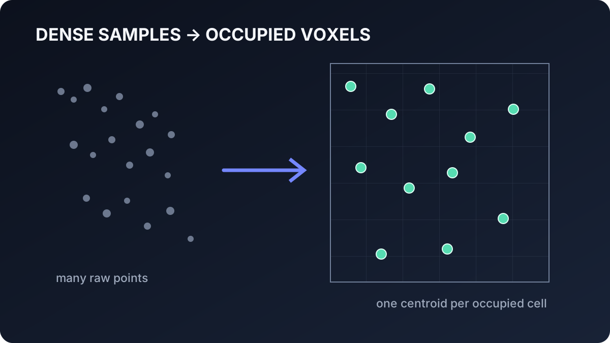
Voxel downsampling reduces a dense point cloud by replacing samples in each occupied 3D cell with their centroid. Learn how voxel indexing and averaging work, how voxel size trades geometric detail for speed, and how to use the filter in the Telekinesis Agentic OS.
Read tutorial →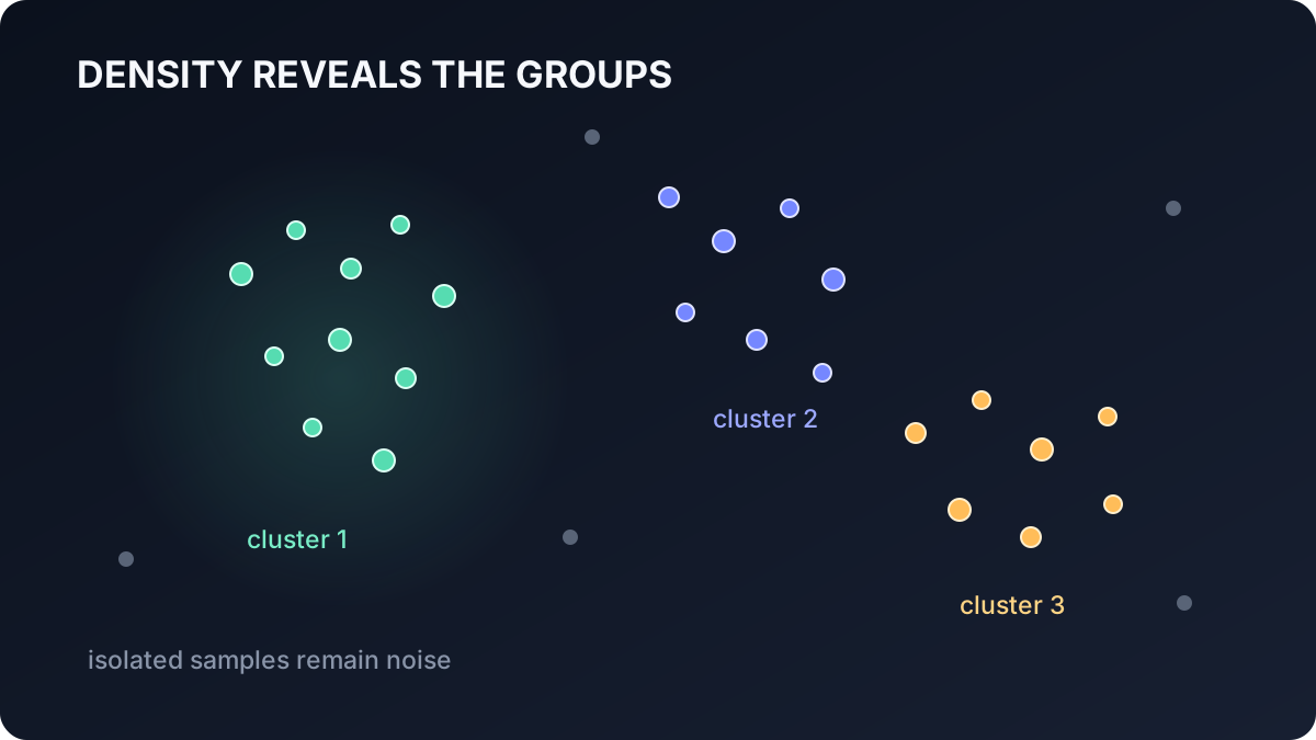 Intermediate · 10 min read
What is DBSCAN Point-Cloud Clustering?
DBSCAN separates a point cloud into dense connected groups without requiring the number of clusters in advance. Learn core, border, and noise points, density reachability, parameter tuning, computational trade-offs, and how to use DBSCAN in the Telekinesis Agentic OS.
Read tutorial →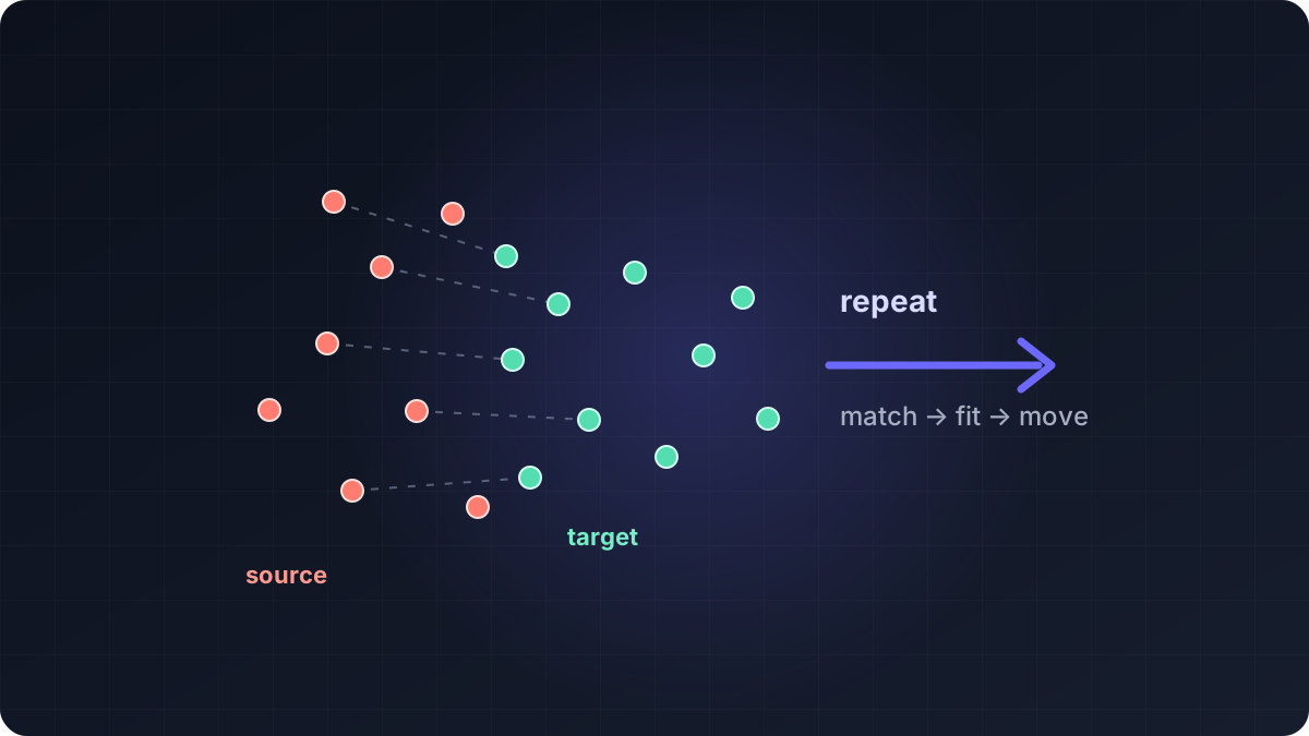 Advanced · 17 min read
What is Iterative Closest Point (ICP)?
Point-cloud registration solves the problem of placing two 3D scans in the same coordinate frame, and ICP does this by repeatedly matching nearby points and fitting a rigid transform. Learn point-to-point and point-to-plane ICP, Fast Global Registration, their mathematics and failure modes, and how to build a coarse-to-fine registration pipeline in the Telekinesis Agentic OS.
Read tutorial →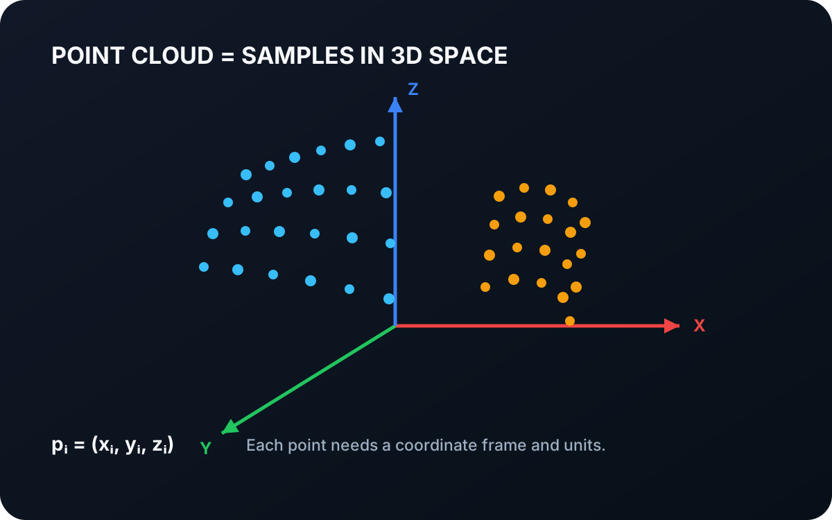 Basic · 4 min read
What is a Point Cloud?
A point cloud is a collection of sampled positions in three-dimensional space. Learn how points represent visible geometry, why coordinate frames matter, and how depth images become spatial data for robots.
Read tutorial →5. References
- Telekinesis. “Filter Point Cloud Using Pass Through Filter”, Vitreous Skill documentation.