Imagine that a robot has a CAD-derived point cloud of a metal bracket and a fresh scan from a depth camera. Both clouds describe the same part, but they sit in different coordinate frames. Until the robot finds the rotation and translation between them, it cannot compare the scan with the model, report the part’s pose, or place a tool accurately.
1. What is Point-Cloud Registration?
Point-cloud registration is the process of finding the spatial transformation that brings two overlapping 3D point sets into alignment. The moving cloud is usually called the source and the reference cloud the target. The result is a transform that expresses source points in the target frame.
Iterative Closest Point (ICP) is the best-known local registration method. It begins from a rough alignment, guesses which source and target points correspond, fits a rigid transform to those pairs, moves the source, and repeats. The name is almost the complete algorithm: the correspondences are chosen iteratively from nearby points.
That simple loop is powerful, but the word local matters. If the initial pose is close enough, nearest points are useful approximations to the unknown physical correspondences. If the clouds begin far apart, the nearest points may belong to unrelated surfaces, and ICP can confidently converge to the wrong pose.
This is why a practical robotics pipeline often has two stages. Fast Global Registration (FGR) uses geometric features to estimate a coarse pose without requiring the clouds to start together. ICP then uses the actual surface geometry to refine that pose. FGR answers “roughly where does this scan belong?”; ICP answers “what small rigid motion makes these overlapping surfaces agree?”
1.1 The Complete Coarse-to-Fine Workflow
Two point clouds → one shared coordinate frame
Global feature matching supplies the basin of attraction; local ICP uses dense surface geometry to obtain the final precision.
Registration begins with two point clouds expressed in different coordinate frames. The source is the cloud we will move. The target is the reference it should align with. If their starting poses are far apart, simply pairing each source point with its nearest target point can create completely wrong correspondences.
The workflow therefore prepares both clouds before alignment. Downsampling reduces cost and makes density more even. Surface normals describe which way the local geometry faces, while FPFH descriptors summarize the shape around selected points. Those descriptors let similar regions propose matches even when the clouds are initially far apart.
Fast Global Registration uses the proposed feature matches to estimate a coarse rigid pose while rejecting many inconsistent pairs. This first transform only needs to bring the clouds into the same neighborhood. Once they are close, ICP can discard the descriptors and alternate between finding nearby geometric correspondences and updating the rotation and translation.
The final transform is still only the optimizer’s best answer. Validation checks whether enough well-distributed points agree, whether the residual error is acceptable, and whether the overlap makes physical sense. Only then should the registered geometry enter a robot-planning pipeline. The following sections build this coarse-to-fine story from the transformation matrix upward.
1.2 What the 4×4 Transformation Matrix Means
Rigid registration estimates a rotation and translation. For a source point , its transformed position is
Here, is source point ; is a rotation matrix; is a translation vector; and is the source point expressed in the target frame. means that preserves lengths and angles and has determinant , so the optimizer cannot scale or mirror the object.
Robotics software usually combines these terms into a homogeneous matrix:
is the complete rigid transform, while the final coordinate value of 1 makes translation possible through matrix multiplication. The matrix is directional: a transform that maps source → target cannot be silently used as target → source. Its inverse performs the opposite mapping.
1.3 The ICP Loop: Match, Fit, Move, Repeat
Suppose the current transform estimate is at iteration . One ICP iteration has four steps:
input: source P, target Q, initial transform T, distance gate d_max

repeat until convergence or max_iterations:
    P_moved ← transform(P, T)
    pairs   ← nearest_target_neighbors(P_moved, Q)
    pairs   ← discard pairs farther than d_max
    ΔT      ← fit_rigid_update(pairs, chosen_error_metric)
    T       ← ΔT · T

return T
The correspondence step treats the pose as fixed. The fitting step treats the correspondences as fixed. Alternating makes a difficult joint problem manageable, but it also explains ICP’s sensitivity: a poor pose creates poor pairs, and poor pairs create a poor pose update.
Interactive ICP iteration
Watch correspondences and the pose update each other
Closest points are paired using the current pose.
The original method by Besl and McKay established the classic closest-point loop and showed monotonic convergence of its mean-square objective to a local minimum. “Monotonic” means the optimized error does not increase under the method’s assumptions. It does not mean that the minimum is the physically correct alignment.
1.4 How Closest-Point Correspondences Are Built
Let the source cloud be and the target cloud be . For each transformed source point, basic ICP chooses the nearest target point:
and are the numbers of source and target points; is the target index assigned to source point ; and is Euclidean distance. A spatial index such as a k-d tree avoids comparing every source point with every target point.
Real clouds only overlap partially, so the nearest point is not automatically a valid match. A maximum correspondence distance rejects pair when
where is the distance gate in the point cloud’s own units. A large gate keeps more overlap but also accepts unrelated geometry. A small gate rejects outliers but may leave too few pairs when the initial pose is rough. Coarse-to-fine registration often begins with a wider gate and reduces it for final refinement.
Point density matters too. If one scan samples a flat surface much more densely, it can contribute many nearly identical pairs and dominate the least-squares fit. Voxel downsampling helps equalize this influence while also reducing the cost of neighbor searches.
1.5 Point-to-Point ICP Fits Paired Samples
Point-to-point ICP minimizes the Euclidean displacement between every accepted source point and its matched target point:
is the total squared registration error; is the set of accepted source indices; is an optional correspondence weight; and the other symbols retain their definitions above. With , the rigid update has a closed-form solution: subtract both point-set centroids, use the cross-covariance of paired points to recover the optimal rotation with singular value decomposition, then align the centroids with translation.
This objective is easy to understand and requires no surface normals. It works well for structured clouds, sharp geometry, or similar sampling. Its weakness is that the target is a surface, but the objective sees only discrete samples of that surface. Two scans can describe the same smooth plane while their sample points do not land at identical locations. Point-to-point ICP spends effort pulling one sample toward another even when both already lie on the same physical surface.
1.6 Point-to-Plane ICP Fits the Local Surface
Point-to-plane ICP changes what counts as error. At target point , let be a unit surface normal. Instead of measuring the full vector between paired points, it projects that vector onto the normal:
is the signed distance from transformed source point to the target’s local tangent plane; is the plane normal; and is the weighted sum of squared normal distances. Motion along the plane is ignored in the local approximation because it does not move the source away from the underlying surface.
Interactive residual geometry
Move one source point along and away from a surface
What to notice: sliding parallel to the local plane increases Euclidean distance, but not the signed normal distance. Point-to-plane ICP therefore models the nearby surface rather than insisting on one exact sampled point.
Chen and Medioni introduced this surface-oriented view for registering range images. It can converge in fewer iterations on smooth surfaces because its local objective better approximates surface-to-surface distance. But it adds a dependency: the target normals must be meaningful.
Normals are usually estimated from a neighborhood around each target point. If is the neighborhood centroid, the local covariance is
is the number of neighboring target points and is a covariance matrix. The eigenvector associated with the smallest eigenvalue points in the direction of least local variation, which is the estimated normal. A tiny neighborhood follows noise; an oversized neighborhood smooths across edges and small features. This is the engineering meaning of normal_search_radius and normal_max_neighbors.
For a small pose update, rotation can be linearized. Let be a small rotation vector and a small translation. Then
The symbol is the 3D cross product. Substituting this approximation into each point-to-plane residual makes it linear in the six unknown pose increments . One least-squares solve produces the next incremental transform. Because the approximation assumes a small update, point-to-plane ICP still needs a reasonable starting pose.
1.7 Why Normals and Geometry Can Make the Pose Unobservable
Registration needs geometry that constrains all six rigid degrees of freedom. A single infinite plane constrains translation along its normal and two rotations, but motion within the plane and rotation around its normal leave the same plane unchanged. The optimizer’s normal equations then become poorly conditioned.
This is not a software bug. The measurements simply do not contain enough information. Corners, intersecting planes, curved surfaces, holes, and asymmetric features add constraints. A symmetric cylinder still leaves rotation around its axis ambiguous; a sphere leaves every rotation ambiguous. If the robot must recover that missing degree of freedom, add another view, include color or learned features, use a known fixture, or carry a prior from odometry.
1.8 Outliers, Partial Overlap, and Robust Kernels
Least squares gives large residuals disproportionate influence because the penalty grows as . That is undesirable when points come from clutter, occlusion, moving objects, or non-overlapping model regions. A robust objective replaces the square with a loss :
is a robust loss such as Tukey’s biweight; is a point-to-point distance or signed point-to-plane residual; and is the assumed noise scale. Small residuals remain influential, while sufficiently large residuals are downweighted or capped.
The noise scale is not a generic “accuracy” control. If is far too large, outliers look ordinary and keep their influence. If it is too small, legitimate correspondences are suppressed before the pose has converged. Robust kernels complement geometric gates; they do not rescue a completely wrong initialization.
1.9 Fast Global Registration Finds the Coarse Pose
ICP searches locally because it pairs points by spatial proximity. FGR starts differently: it describes local geometry around downsampled points, then matches points whose descriptors look alike even when their coordinates are far apart.
The Telekinesis Skill computes surface normals and Fast Point Feature Histograms (FPFH). An FPFH descriptor summarizes angular relationships between a point’s normal and neighboring normals. It is designed to be more stable under rigid motion than raw coordinates, so a corner on the source model can be proposed as a match for a similar corner in the target scan.
Descriptor matches contain outliers. Repeated holes, flat regions, and similar corners can produce plausible but false pairs. FGR’s central contribution is to optimize one robust objective over the candidate matches rather than repeatedly sampling small match sets as RANSAC does:
is the set of candidate feature correspondences; identifies one candidate source–target pair; and is a robust Geman–McClure-style penalty controlled by scale . Through an equivalent line process, every pair receives a weight
lies between 0 and 1. A geometrically consistent match keeps a high weight; a large-residual match approaches zero. FGR alternates between updating these weights and updating the pose.
Interactive robust matching
See how FGR keeps useful feature matches and suppresses outliers
Small μ is selective: only already-consistent matches keep much weight. Graduated non-convexity begins with a smoother objective and lowers μ so bad matches lose influence as the pose improves.
The optimization uses graduated non-convexity. It starts with a large , creating a smoother problem in which the optimizer can make broad progress. It then reduces , making the loss more selective so inconsistent matches lose influence. The candidate set stays fixed during the inner optimization, so FGR avoids repeated closest-point searches.
FGR is global in the practical sense that it does not require an already-close pose. It does not guarantee the globally optimal answer for every scene. Repeated geometry, weak features, low overlap, or incorrect scale can still defeat it. Its output should be treated as an initialization and validated or refined.
1.10 Choosing the Right Stage
| Method | Correspondence cue | Error being minimized | Needs a close initial pose? | Best role |
|---|---|---|---|---|
| Fast Global Registration | Similar FPFH descriptors | Robust distance over feature matches | No rough pose required | Coarse alignment |
| Point-to-point ICP | Spatial nearest neighbor | Euclidean point distance | Yes | Simple local refinement |
| Point-to-plane ICP | Spatial nearest neighbor + target normal | Signed tangent-plane distance | Yes | Fast, accurate surface refinement |
Use point-to-point ICP when normals are unavailable or unreliable, or when distinct sampled geometry provides good constraints. Use point-to-plane ICP when the target has clean surface normals and smooth overlap. Use FGR when no trustworthy initial transform exists, then refine its result with ICP at full or progressively finer resolution.
1.11 When Registration Fails
The residual alone can be deceptive. A model can align neatly with the wrong repeated feature and still achieve a small error. Build validation around the task:
- Overlap: require enough accepted correspondences distributed across the object, not concentrated on one small patch.
- Residual distribution: inspect median and tail errors, not only the mean or RMSE.
- Pose plausibility: reject translations, rotations, or frame directions that violate the robot cell’s physical limits.
- Geometric conditioning: detect when flat or symmetric geometry leaves a degree of freedom weakly constrained.
- Repeatability: perturb the initial pose or resample the cloud; a stable solution should return to nearly the same transform.
- Task outcome: measure pick, inspection, or localization success after registration. A low point error is not automatically a useful tool pose.
2. How to Use Registration in the Telekinesis Agentic OS
Telekinesis exposes all three stages as Vitreous Skills. The following example shows the intended coarse-to-fine structure. Distances are illustrative: they must be scaled to the units, point spacing, and expected pose error of your clouds.
import numpy as np
from telekinesis import vitreous

# Coarse alignment from local geometric features.
coarsely_aligned = vitreous.register_point_clouds_using_fast_global_registration(
    source_point_cloud=source_point_cloud,
    target_point_cloud=target_point_cloud,
    initial_transformation_matrix=np.eye(4),
    normal_radius=0.02,
    normal_max_neighbors=20,
    feature_radius=0.05,
    feature_max_neighbors=30,
    max_correspondence_distance=0.015,
)
The FGR Skill currently returns a registered point cloud. The ICP Skills return a transformation matrix, which you apply separately. If you already have a rough transform from calibration, odometry, a fixture, or another registration stage, point-to-point refinement is direct:
point_to_point_transform = vitreous.register_point_clouds_using_point_to_point_icp(
    source_point_cloud=source_point_cloud,
    target_point_cloud=target_point_cloud,
    initial_transformation_matrix=rough_transform,
    max_iterations=100,
    max_correspondence_distance=0.02,
    use_robust_kernel=True,
    loss_type="tukey_loss",
    noise_standard_deviation=0.005,
)

aligned_source = vitreous.apply_transform_to_point_cloud(
    point_cloud=source_point_cloud,
    transformation_matrix=point_to_point_transform,
)
For a clean target surface with useful normals, switch to point-to-plane refinement:
point_to_plane_transform = vitreous.register_point_clouds_using_point_to_plane_icp(
    source_point_cloud=source_point_cloud,
    target_point_cloud=target_point_cloud,
    initial_transformation_matrix=rough_transform,
    max_iterations=100,
    max_correspondence_distance=0.02,
    normal_search_radius=0.01,
    normal_max_neighbors=30,
    use_robust_kernel=True,
    loss_type="tukey_loss",
    noise_standard_deviation=0.005,
)
Parameter values must share the cloud’s units. In a cloud measured in metres, 0.02 means two centimetres; in millimetres it means two hundredths of a millimetre. Confirm units before tuning anything.
2.1 A Practical Tuning Order
- Confirm both clouds use the same units and scale.
- Remove obvious outliers and isolate the object or overlapping scene region.
- Choose a voxel size that preserves task-critical geometry.
- Set the normal radius to cover several point spacings without crossing unrelated surfaces.
- Set the FPFH feature radius larger than the normal radius so descriptors see enough local shape.
- Run FGR when the initial pose is unknown.
- Begin ICP with a correspondence gate wide enough for the coarse pose error, then tighten it.
- Enable a robust kernel when partial overlap or clutter remains.
- Validate the transform with held-out geometry and the downstream robot task.
Do not tune max_iterations first. If correspondences are wrong, more iterations merely optimize the wrong problem for longer. Fix preprocessing, initialization, neighborhood scale, and distance gates before increasing the iteration budget.
3. How to Benchmark a Registration Pipeline
The classic papers answer different questions. Besl and McKay established the behavior of the local closest-point loop over several geometric representations. Chen and Medioni demonstrated surface-based registration of multiple range images. Zhou, Park, and Koltun evaluated FGR as a fast global initializer and reported that it matched or exceeded the accuracy of contemporary global pipelines while running at least an order of magnitude faster in their experiments. Those results explain the algorithms; they do not predict latency or accuracy for a hosted Skill on your point clouds.
For a robot deployment, benchmark the complete pipeline:
| Metric | Definition | What it reveals |
|---|---|---|
| Rotation error | Angle of | Orientation accuracy |
| Translation error | Position accuracy in physical units | |
| Inlier RMSE | RMSE over gated correspondences | Local surface fit |
| Fitness / overlap | Fraction of points with valid matches | How much geometry supports the pose |
| Recall at tolerance | Fraction of trials below pose thresholds | Reliability across scenes |
| End-to-end latency | Transfer + preprocessing + registration + validation | Whether the pipeline meets the robot cycle time |
| Task success | Successful picks, insertions, or inspections | Whether geometric accuracy is operationally sufficient |
Evaluate easy and adversarial cases separately: high and low overlap, clean and noisy depth, symmetric objects, clutter, occlusion, different initial rotations, and target-absent scenes. Report failures rather than averaging them away. Registration is most dangerous when it produces a plausible transform for an invalid match.
4. Where to Go Next
 Basic · 4 min read
What is a Point Cloud?
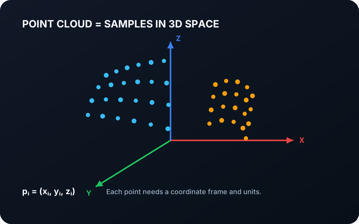
A point cloud is a collection of sampled positions in three-dimensional space. Learn how points represent visible geometry, why coordinate frames matter, and how depth images become spatial data for robots.
Read tutorial →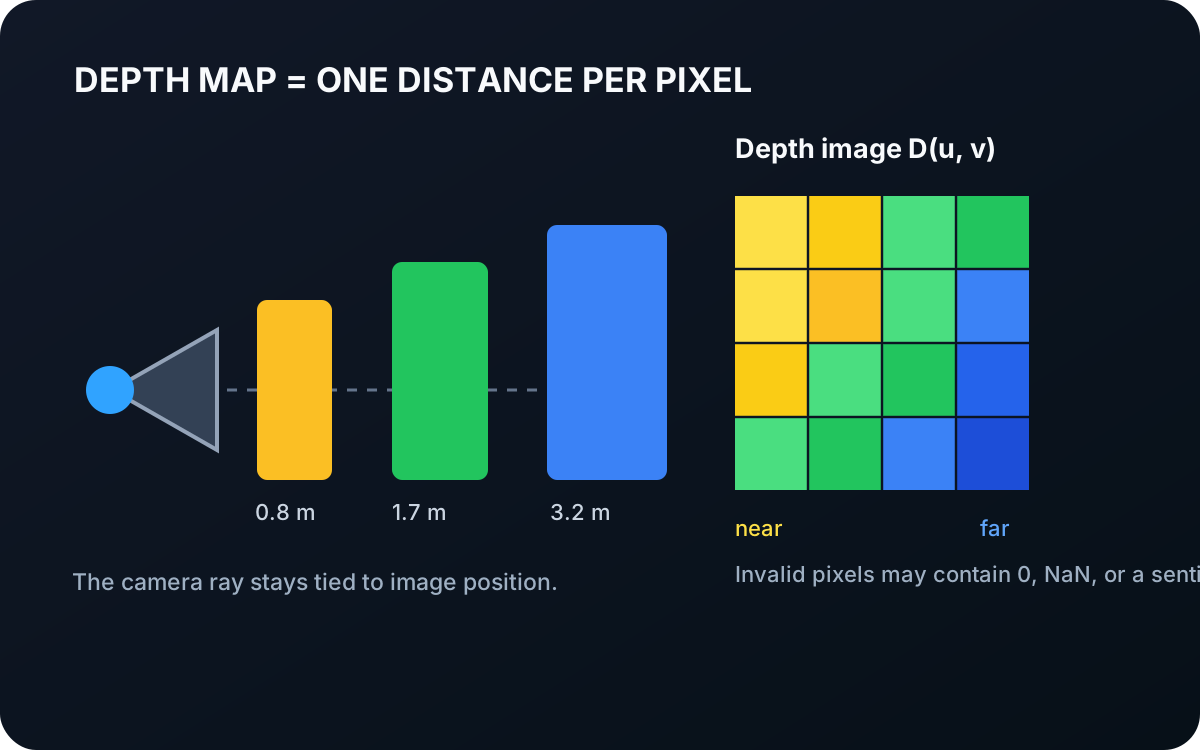 Basic · 4 min read
What is a Depth Map?
A depth map stores an estimated distance for each image position. Learn how depth remains aligned with pixels, how it differs from color, and how calibration converts it into 3D geometry.
Read tutorial →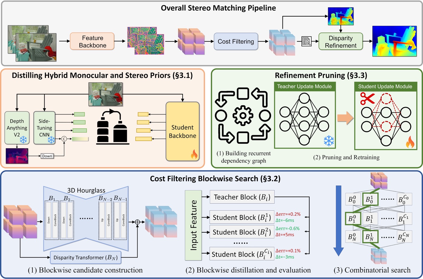 Intermediate · 15 min read
What is Fast-FoundationStereo?
Fast-FoundationStereo solves the problem of recovering metric scene depth from two calibrated camera images quickly enough for real-time perception. Learn stereo geometry, its feature–cost–refinement architecture, its training losses, and how to use it in the Telekinesis Agentic OS.
Read tutorial →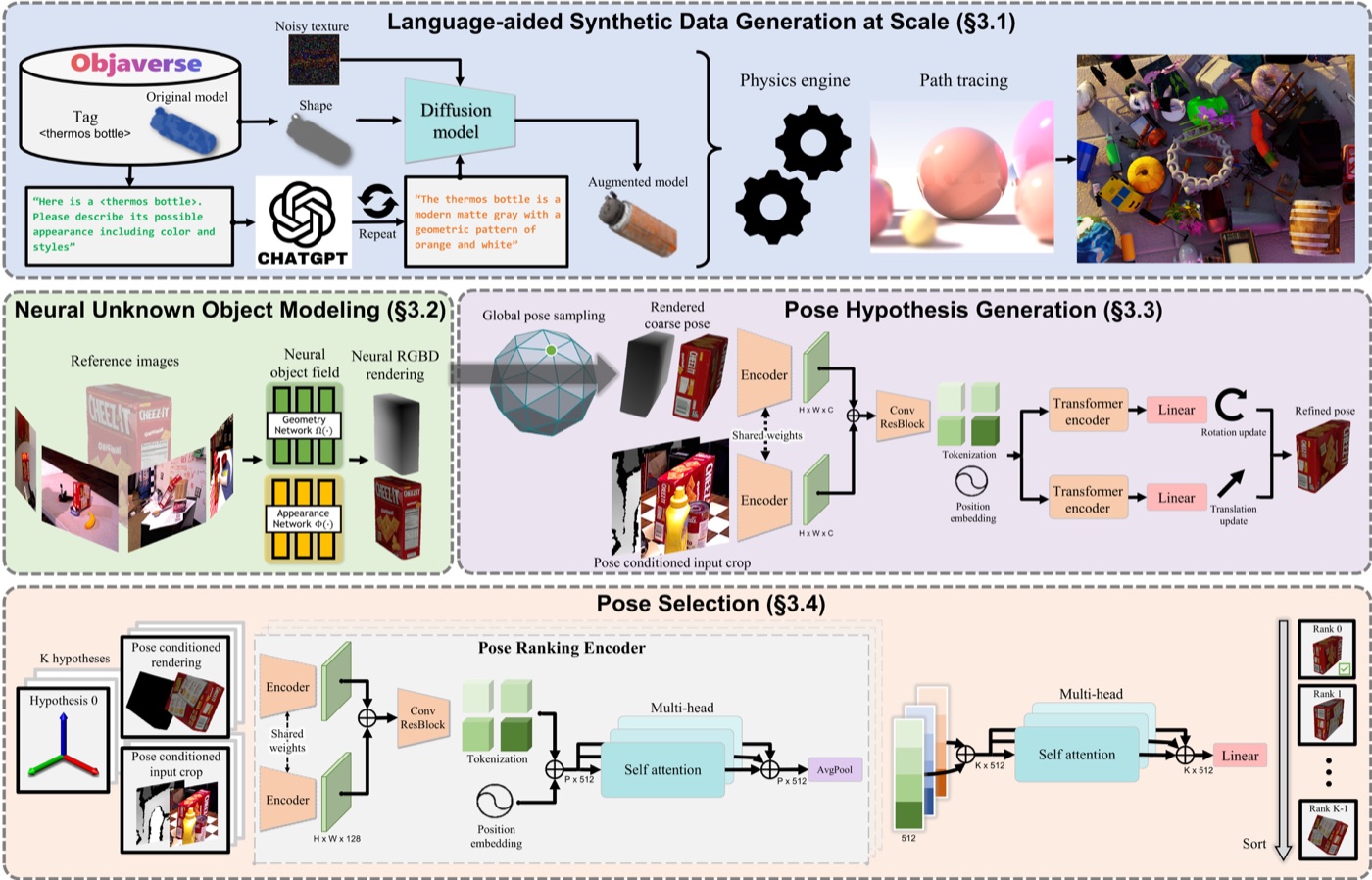 Advanced · 16 min read
What is FoundationPose?
FoundationPose solves the problem of locating a previously unseen rigid object in 3D when its shape is known. Learn how pose hypotheses are rendered, refined, ranked, and tracked, which losses train the model, and how to use it in the Telekinesis Agentic OS.
Read tutorial →5. References
- Besl, P. J., and McKay, N. D. “A Method for Registration of 3-D Shapes”, IEEE Transactions on Pattern Analysis and Machine Intelligence, 1992.
- Chen, Y., and Medioni, G. “Object Modelling by Registration of Multiple Range Images”, Image and Vision Computing, 1992.
- Zhou, Q.-Y., Park, J., and Koltun, V. “Fast Global Registration”, European Conference on Computer Vision, 2016.
- Rusu, R. B., Blodow, N., and Beetz, M. “Fast Point Feature Histograms (FPFH) for 3D Registration”, IEEE International Conference on Robotics and Automation, 2009.
- Telekinesis. “Register Point Clouds Using Point-to-Point ICP”, Vitreous Skill documentation.
- Telekinesis. “Register Point Clouds Using Point-to-Plane ICP”, Vitreous Skill documentation.
- Telekinesis. “Register Point Clouds Using Fast Global Registration”, Vitreous Skill documentation.