Imagine a mobile robot moving through a warehouse. It must notice people, boxes, and vehicles quickly enough to react. YOLOX is an object detector built for this kind of fast visual recognition, and its design is a useful way to learn how modern real-time detection works.
1. What is YOLOX?
Suppose a mobile robot enters a warehouse aisle. One camera frame may contain a person nearby, several cartons at different distances, and a forklift partly hidden at the far end. The robot needs both identity and location: what is present and where it is in the image.
YOLOX is a real-time object detector that returns boxes, class labels, and confidence scores. It belongs to the YOLO family, whose central goal is to perform detection in one fast network pipeline.
YOLOX is described as a one-stage, anchor-free detector. One-stage means it predicts candidates directly from image features instead of using one learned stage to propose regions and another to classify them. Anchor-free means it predicts box geometry without starting from a catalogue of predefined rectangle shapes. Neither term changes the vocabulary: YOLOX still recognizes the classes it learned during training.
The paper develops this pipeline through three connected ideas: anchor-free prediction simplifies where boxes come from, a decoupled head separates the jobs of classification and localization, and SimOTA decides which predictions should learn from each annotated object.
1.1 See the Full YOLOX Pipeline
Image → filtered detections
SimOTA assigns positive locations during training; NMS resolves duplicates during inference.
Read the diagram from top to bottom. Image passes through the CSP backbone, PAN / FPN, and Decoupled head. A Score filter + NMS removes weak and duplicate candidates, leaving the final Detections.
1.2 From Camera Image to Multi-Scale Features
Follow one camera frame from the first diagram box. The Image enters a CSP backbone, a convolutional network that turns pixels into a hierarchy of feature maps. Early, high-resolution maps preserve local detail; deeper maps represent larger patterns and more semantic information.
The next diagram box, PAN / FPN, is the neck that combines features from several resolutions. This matters because the cartons near the robot and the forklift at the end of the aisle occupy very different numbers of pixels. Feature-pyramid representations let small objects use detailed high-resolution features while larger objects use features with wider context.
The Decoupled head then examines many positions across those multi-scale feature maps. At each candidate position it predicts box geometry, objectness, and class evidence. “Dense” simply means that the network checks a regular grid of possible locations rather than beginning with a short list of proposed objects.
1.3 How YOLOX Predicts Boxes Without Anchors
To see why anchor-free prediction matters, consider an older anchor-based detector. At every grid location, it places several template rectangles with predefined widths and aspect ratios. The network learns how to shift and resize them. If the dataset changes from people and cars to long tools and tiny fasteners, those templates may need to be reconsidered.
YOLOX removes the template catalogue. It treats a feature-map location as a possible object centre and directly predicts the distances needed to describe the box. Relative to the paper’s anchor-based baseline, this reduces the predictions at each location from three to one.
The design is simpler, but it is not assumption-free. Input resolution determines how much detail exists, feature strides determine the spatial grid, and the training assignment determines which locations learn each object. Anchor-free removes one family of hand-designed choices; it does not remove the need for sound data and geometry.
1.4 Why Class and Box Predictions Use Separate Branches
Once a candidate location has been chosen, the detector must answer different questions. “What is it?” depends on appearance and semantic cues. “Where exactly does it end?” depends on boundaries and geometry. Those tasks can prefer different features.
YOLOX therefore uses a decoupled head. The branches share the feature pyramid but separate near the output: one branch predicts class evidence, another predicts box geometry, and a third predicts objectness—whether any supported object is present at that location. This reduces direct interference between classification and localization.
A simplified final score can be understood as
This product explains why a location must look both object-like and class-consistent to receive a strong final score. It is a mental model, not a promise that the score is a calibrated probability. Thresholds still need to be validated on the robot’s own camera data.
1.5 What Changed from Earlier YOLO Detectors?
The paper’s contribution is best understood as a careful modernization of a YOLOv3-style baseline. Each change solves a different part of the pipeline: anchor-free prediction simplifies candidate geometry, the decoupled head separates output tasks, and SimOTA improves training assignment. The performance gain comes from making these pieces work together.
1.6 How SimOTA Assigns Training Examples
Dense prediction creates a training ambiguity. Many nearby grid locations may produce boxes around the same annotated person. If all are treated as correct, duplicates dominate. If the wrong location is selected, the model learns from a poor candidate.
SimOTA resolves this in stages. A centre prior first removes implausible distant candidates. For the remaining candidates, the algorithm combines classification and regression losses into a matching cost. It then chooses a dynamic number of low-cost positives for each object. An object with several good candidates can supervise more locations than one with only a few reliable candidates.
This assignment exists only during training. It teaches the dense head which locations should become responsible for which objects. During inference, the trained network directly emits its candidates.
1.7 How Score Filtering and NMS Clean the Results
At inference time, the diagram moves from the Decoupled head to Score filter + NMS. Score filtering first removes candidates whose evidence is too weak. Even among the remaining candidates, neighbouring locations can predict the same physical object. Non-maximum suppression (NMS) sorts those boxes by score, keeps the strongest, and removes weaker boxes that overlap it beyond a chosen threshold. Overlap is measured with intersection over union:
The overlap threshold controls which lower-scoring candidates are removed:
- Lower NMS threshold: suppression is more aggressive; duplicates fall, but close objects may erase each other.
- Higher NMS threshold: more overlapping boxes survive; crowded objects may be retained, but duplicates rise.
This threshold creates a real robotics trade-off. Aggressive suppression removes duplicate boxes but may erase one of two nearby parts. Gentle suppression preserves crowded objects but can leave several boxes around one part. The boxes that survive become the final Detections shown at the bottom of the diagram. NMS finishes detection within a single image; it is not tracking and cannot establish identity across successive camera frames.
1.8 Where YOLOX Can Fail
The whole story now connects. YOLOX extracts multi-scale features, predicts dense anchor-free candidates through separate output branches, and removes duplicate boxes with NMS. This makes it fast and practical, but not infallible.
Small or blurred objects may not leave enough visual evidence. Unseen classes remain outside the learned vocabulary. Crowded objects can interfere during suppression, and a correct 2D box may still be too coarse for grasping. A robot should treat YOLOX as the localization stage of a larger perception system, not as a complete understanding of the scene.
2. How to Use YOLOX in the Telekinesis Agentic OS
Telekinesis provides YOLOX as the Retina Skill detect_objects_using_yolox. The code below loads an image, applies score and non-maximum-suppression thresholds, resolves the COCO category names, and prints each detection.
from telekinesis import constants, datatypes, retina

image = datatypes.Image.from_url(
    url="https://assets.telekinesis.ai/examples/v1/images/warehouse_2.jpg"
)

detections = retina.detect_objects_using_yolox(
    image=image,
    score_threshold=0.80,
    nms_threshold=0.45,
)

categories = constants.get_coco_categories(model="yolox")

for detection in detections:
    label = categories[detection.category_id]
    print(label.name, detection.score, detection.bbox)
The visualization below is the post-NMS result, not the network’s much larger dense candidate set. Compare it against crowded and overlapping scenes when selecting deployment thresholds.
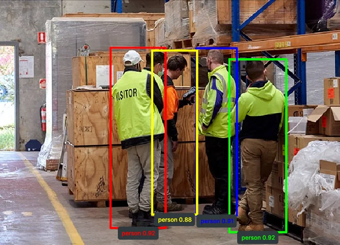
Dense predictions become a short final list only after confidence filtering and suppression of overlapping candidates.
3. Benchmarking
3.1 Results Reported in the YOLOX Paper
Table 3 of the YOLOX paper evaluates 640×640 inputs with FP16 and batch size 1 on a Tesla V100. The numbers compare paper checkpoints under that specific setup.
| Model | COCO AP | Parameters | GFLOPs | Latency |
|---|---|---|---|---|
| YOLOX-S | 39.6 | 9.0M | 26.8 | 9.8 ms |
| YOLOX-M | 46.4 | 25.3M | 73.8 | 12.3 ms |
| YOLOX-L | 50.0 | 54.2M | 155.6 | 14.5 ms |
| YOLOX-X | 51.2 | 99.1M | 281.9 | 17.3 ms |
Retina service performance includes more than paper inference: image transfer, decoding, preprocessing, model execution, NMS, serialization, and network latency. Benchmark the complete call with representative images.
3.2 Comparison with Other Telekinesis Skills
| Skill | Vocabulary | Post-processing control | Prefer it when |
|---|---|---|---|
| YOLOX | Fixed COCO-80 | Score + NMS thresholds | Dense real-time detection and NMS control |
| RF-DETR | Fixed COCO-80 | Score threshold | Transformer set prediction and global context |
| Grounding DINO | Open phrases | Box + text thresholds | Categories change at inference time |
| Qwen | Requested names | Object list | Broader semantic interpretation is needed |
3.3 YOLOX, RF-DETR, and Open-Vocabulary Detectors
YOLOX is a strong choice when the fixed COCO vocabulary fits, latency matters, and explicit NMS tuning is useful. RF-DETR offers transformer set prediction and stronger global interaction. Grounding DINO accepts changing text prompts, but prompt design and open-vocabulary calibration become new variables.
Benchmark them as complete pipelines. Model inference speed alone omits image transfer, decoding, preprocessing, post-processing, and network latency. Record median and tail latency, detection quality by scenario, and final robot task success.
4. Where to Go Next?
Compare the same frames with RF-DETR. If boxes are too coarse for the task, study image segmentation; if the target class is unknown at training time, use Grounding DINO.
5. References
- Ge, Z., Liu, S., Wang, F., Li, Z., and Sun, J. “YOLOX: Exceeding YOLO Series in 2021”, 2021.
- Redmon, J. et al. “You Only Look Once: Unified, Real-Time Object Detection”, CVPR, 2016.
- Lin, T.-Y. et al. “Feature Pyramid Networks for Object Detection”, CVPR, 2017.
- Bodla, N. et al. “Soft-NMS—Improving Object Detection With One Line of Code”, ICCV, 2017.