Imagine a robot watching parts move along a conveyor. Its detector must find each part accurately, but it must also respond before the part has moved away. RF-DETR is designed to help engineers find that balance between detection accuracy and speed.
1. What is RF-DETR?
Return to the conveyor example. If the camera captures 30 frames each second but detection takes half a second, the robot is always reacting to the past. A smaller model may respond on time but miss difficult parts. The useful detector is not simply the most accurate one—it is the most accurate one that meets the system’s timing budget.
RF-DETR is a real-time specialist detection transformer built around that trade-off. It looks at an image and produces a set of labeled boxes. Specialist means the model is adapted to the classes needed by a target task. Real-time means latency is treated as a design objective rather than checked only after training.
RF-DETR is therefore different from an open-vocabulary detector. It does not accept any new phrase and immediately understand a new class. Instead, it asks a deployment-focused question: once a detector has learned the target domain, which model configuration gives the best accuracy on the available hardware without responding too slowly?
1.1 See the Full RF-DETR Pipeline
Image + object queries → prediction set
Weight-sharing search varies the backbone and decoder configuration, then selects a point on the accuracy–latency frontier.
Read the diagram from top to bottom. Image and learned Object queries enter the detector. Image features pass through the DINOv2 backbone and Feature projector. The DETR decoder combines those features with the queries and produces a Prediction set of classes and boxes.
1.2 From an Image and Object Queries to Predictions
The diagram begins at Image. A pretrained DINOv2 backbone converts it into visual tokens that describe the scene. The Feature projector then reshapes those backbone features into the representation expected by the decoder.
The second input is Object queries. Following the set-prediction idea introduced by DETR, the model begins with a fixed collection of learned prediction slots rather than a dense list of overlapping candidate boxes.
Picture the queries as a row of empty inspection forms. After the decoder studies the image features, one form may contain “worker” and a box, another may contain “forklift” and a box, and the remaining forms may say “no object.” The queries are not permanently tied to particular classes; they are reusable slots that compete to explain what is present in the current image.
The DETR decoder brings both streams together. Each query attends to the projected image features and is refined into a class and box, or into “no object.” The final Prediction set contains the useful query results.
1.3 How Each Query Learns One Object
Set prediction creates one important training problem. Predictions have no natural order. The first query is not guaranteed to describe the first annotated object, so the loss cannot simply compare row one with row one.
DETR solves this using the assignment method introduced by Kuhn. It finds a one-to-one pairing between predicted slots and annotated objects that minimizes a matching cost. Conceptually, that cost is
The three terms ask complementary questions. Does the predicted class match? Are the box coordinates close? Do the boxes overlap geometrically? Once the lowest-cost pairing is found, every matched query learns from one object and every unmatched query learns “no object.” The one-to-one structure discourages several queries from claiming the same target.
The overlap term begins with intersection over union:
IoU is one when boxes match perfectly and zero when they do not overlap. The zero case is awkward during learning because it provides little guidance about how the prediction should move. Generalized IoU also considers the smallest box enclosing both regions, providing a useful signal even before the boxes touch.
1.4 How RF-DETR Balances Accuracy and Speed
So far, this explains how RF-DETR detects objects. Its distinctive contribution is how it searches for a deployable version of that detector.
Training every possible architecture independently would be prohibitively expensive. RF-DETR instead trains a weight-sharing super-network. Think of it as one large network that contains many smaller valid subnetworks. Those subnetworks reuse learned weights, allowing thousands of candidate configurations to be evaluated without starting training from zero each time.
The search varies choices such as image resolution, patch size, windowed attention, decoder depth, and query count. Increasing one of these may improve accuracy but also add computation. The goal is not to find one universally best configuration. It is to recover an accuracy–latency curve for the target dataset and platform.
Along that curve, the Pareto frontier contains configurations for which no alternative is both faster and more accurate. An engineer can select the point that satisfies the robot’s timing budget. Because runtime depends on the accelerator, numerical precision, batch size, and inference engine, that choice must be measured on the actual deployment stack.
1.5 Where RF-DETR Can Fail
- Domain shift: deployment imagery can differ from the detector’s fine-tuning distribution.
- Small objects: limited pixels and feature resolution reduce class and box evidence.
- Occlusion and crowds: nearby instances may be missed or localized poorly.
- Look-alike classes: visually similar categories can exchange confidence.
- Motion blur and exposure: an otherwise familiar object loses usable texture.
- Box insufficiency: a correct rectangle still includes background and says nothing about graspable geometry.
These limitations connect back to the original story. Architecture search can help a conveyor detector respond faster without giving up unnecessary accuracy, but it cannot restore detail lost to blur, reveal a fully hidden part, or teach a class absent from the training data. A correct box also remains only a 2D region; manipulation still requires depth, shape, calibration, and safety checks.
2. How to Use RF-DETR in the Telekinesis Agentic OS
Telekinesis provides RF-DETR as the Retina Skill detect_objects_using_rfdetr. The code below loads an image, applies a score threshold, resolves the COCO category IDs, and converts one returned box from width–height form to corner coordinates.
from telekinesis import constants, datatypes, retina

image = datatypes.Image.from_url(
    url="https://assets.telekinesis.ai/examples/v1/images/warehouse_1.jpg"
)

detections = retina.detect_objects_using_rfdetr(
    image=image,
    score_threshold=0.50,
)

categories = constants.get_coco_categories(model="rfdetr")

for detection in detections:
    category = categories[detection.category_id]
    x, y, width, height = detection.bbox
    print(category.name, detection.score, (x, y, width, height))
# Convert Retina's [x, y, width, height] box to corner coordinates.
x_min, y_min, width, height = detection.bbox
x_max = x_min + width
y_max = y_min + heightThe output image shows the final prediction set after thresholding. Use it to check class identity and box coverage before connecting a detection to depth, tracking, or manipulation logic.
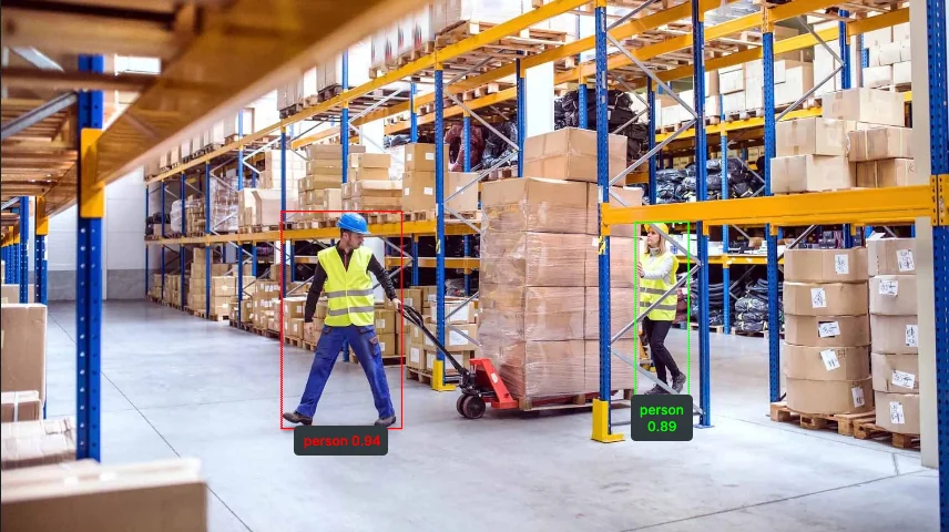
A box localizes image extent; it does not provide depth, 6D pose, free space, or a safe grasp.
3. Benchmarking
3.1 Results Reported in the RF-DETR Paper
The RF-DETR paper evaluates COCO using TensorRT 10.4 on an NVIDIA T4 and reports latency with the same model artifact used for accuracy. Selected rows from Table 2 are shown below.
| Model | Size | Parameters | Latency | COCO AP | AP50 |
|---|---|---|---|---|---|
| D-FINE | Nano | 3.8M | 2.1 ms | 42.7 | 60.2 |
| RF-DETR | Nano | 30.5M | 2.3 ms | 48.0 | 67.0 |
| D-FINE | Small | 10.2M | 3.5 ms | 50.6 | 67.6 |
| RF-DETR | Small | 32.1M | 3.5 ms | 52.9 | 71.9 |
| RF-DETR | Medium | 33.7M | 4.4 ms | 54.7 | 73.5 |
| RF-DETR | 2XL | 126.9M | 17.2 ms | 60.1 | 78.5 |
These figures are not Retina service latency. Network transport, serialization, input resolution, service artifact, and concurrency must be measured end to end in your Agentic OS deployment.
3.2 Comparison with Other Telekinesis Skills
| Property | RF-DETR | YOLOX |
|---|---|---|
| Core formulation | Transformer set prediction | Dense, one-stage anchor-free prediction |
| Global context | Native attention-based reasoning | Primarily convolutional feature hierarchy |
| Duplicate handling | Trained toward unique set predictions | Explicit NMS exposed by Retina |
| Retina tuning | Score threshold | Score and NMS thresholds |
| Label vocabulary | Fixed COCO classes | Fixed COCO classes |
Neither architecture wins every scene. RF-DETR may benefit from global relationships and the DETR formulation; YOLOX offers direct control over duplicate suppression and a mature one-stage design. Evaluate accuracy, tail latency, memory, and failure consistency on the same recorded frames.
4. Where to Go Next?
Study YOLOX to understand one-stage anchor-free detection and NMS. If the required class is outside COCO, continue with Grounding DINO.
5. References
- Robinson, I., Robicheaux, P., Popov, M., Ramanan, D., and Peri, N. “RF-DETR: Neural Architecture Search for Real-Time Detection Transformers”, 2025.
- Carion, N. et al. “End-to-End Object Detection with Transformers”, ECCV, 2020.
- Rezatofighi, H. et al. “Generalized Intersection over Union: A Metric and a Loss for Bounding Box Regression”, CVPR, 2019.
- Lin, T.-Y. et al. “Microsoft COCO: Common Objects in Context”, ECCV, 2014.