Suppose a robot must separate dark hardware from a pale background, but the histogram does not form two clean bell-shaped peaks. Otsu’s variance criterion may place the split somewhere unhelpful. Yen thresholding gives the engineer a second automatic hypothesis by asking a different statistical question about the same histogram.
1. What is Yen Thresholding?
Yen thresholding is an automatic global-threshold algorithm that selects the histogram split maximizing a probability-concentration criterion. It solves the same broad task as Otsu—choose one cutoff without manual tuning—but it ranks candidate thresholds using different statistics.
The method comes from Yen, Chang, and Chang’s 1995 paper, “A New Criterion for Automatic Multilevel Thresholding”. The binary version evaluates every possible division into a lower-intensity and upper-intensity class.
1.1 The Complete Yen Pipeline
Histogram → maximum correlation criterion → mask
Yen optimizes a probability-concentration criterion rather than Otsu’s variance separation, so the two methods can choose different thresholds from the same histogram.
Yen thresholding also chooses one global cutoff from the image rather than asking the engineer to supply it. It starts by counting the gray levels and converting those counts into probabilities, so common intensities carry more weight than rare ones.
The method then places a possible threshold at every gray level. Each placement creates a darker class and a brighter class. Yen’s criterion scores that split using both the probability contained in each class and how concentrated those probabilities are. The threshold with the best score is selected.
Only after this search does the algorithm return to the image. Every pixel is compared with the winning cutoff to create the binary mask. The scoring rule differs from Otsu’s variance-based rule, so the two methods can choose different splits from the same histogram.
Like Otsu, Yen has no access to pixel position while choosing the threshold. A dark cluster in the image corner and a dark object in the center contribute to the same histogram bins. Connectivity and shape must be checked after thresholding.
1.2 Start With Histogram Probabilities
Let be the number of pixels at gray level , and let be the total pixel count. The normalized histogram is
is the number of possible intensity levels, and is the probability of intensity . For candidate threshold , the lower class probability is
while the upper class has probability . Yen’s calculation additionally uses squared-probability sums:
and become large when probability mass within a class is concentrated in fewer bins and smaller when it is diffuse across many bins.
1.3 The Yen Criterion
A commonly implemented binary form scores each valid threshold as
is the Yen score, is the natural logarithm, and the other symbols are the cumulative quantities defined above. Thresholds that create empty classes or zero-valued logarithm arguments are excluded or handled numerically. The selected threshold is
is then applied globally to the image. The criterion arises from an entropic/correlation treatment of the two classes. The important engineering insight is not to memorize the logarithms; it is to understand that Yen rewards different histogram structure from Otsu.
Interactive Yen objective
Change the class balance and inspect the selected split
Intensity histogram
Objective for every candidate threshold
1.4 How Yen Differs From Otsu
Otsu uses class weights and class means to maximize between-class variance. Yen uses cumulative probabilities and their squared sums. Therefore two images—or even one histogram—can lead to different thresholds.
Otsu is compelling when two intensity populations are compact and their means are well separated. Yen can be a useful alternative when probability concentration and tails produce a better split than the variance criterion. Neither method dominates universally, and “try both” should mean compare both on labeled deployment data, not choose the prettier single example.
| Property | Otsu | Yen |
|---|---|---|
| Candidate input | Same normalized histogram | Same normalized histogram |
| Main statistics | Class weights and means | Class probability and squared-probability sums |
| Objective | Maximum between-class variance | Maximum Yen criterion |
| Output | One global threshold | One global threshold |
| Spatial awareness | None | None |
1.5 Why an Automatic Threshold Can Still Be Wrong
The optimizer always answers the mathematical problem it was given. That problem may not match the robot’s task. A large shadow can become one class and the rest of the scene another. Background texture can dominate the histogram. A tiny defect can be statistically invisible. A target-absent scene still has an intensity distribution and still yields a threshold.
This is the central safety lesson of automatic thresholding: parameter-free does not mean assumption-free. Yen assumes that a useful binary partition is expressed in the global intensity histogram.
1.6 Global Illumination Remains Global
Yen adapts from frame to frame, but it still returns one number per frame. If brightness varies spatially, one threshold may over-segment the bright side and under-segment the dark side.
Use a crop when irrelevant areas distort the histogram. Use local/adaptive thresholding when the cutoff genuinely changes across the image. Improve illumination when the workcell can be engineered. Algorithm choice should follow the physical cause of the intensity variation.
1.7 Criterion Versus Training Loss
Yen’s is an optimization criterion, not a learned-model loss. The method has no weights, training set, gradient descent, or post-training inference phase. It searches a small discrete set of thresholds for each image.
Evaluation happens outside that criterion. For ground-truth mask and prediction , measure IoU, precision, and recall. If the downstream operation picks a centroid, report centroid error. If it counts parts, report count accuracy. A high internal Yen score is not a substitute for those task metrics.
1.8 Efficient Computation
A naive implementation could recompute every sum for every threshold. Cumulative arrays make the scan efficient: calculate and from left to right, calculate the complementary squared sum for the upper class, then evaluate at each gray level.
For an eight-bit image, the histogram has only 256 bins. Histogram construction scales with the number of pixels, while candidate evaluation scales with the number of bins. In a Telekinesis pipeline, image transport and serialization may matter more than the threshold calculation itself, so benchmark the complete call.
1.9 A Practical Comparison Protocol
Collect images covering all valid brightness, target sizes, and target-absence cases. Apply manual, Otsu, and Yen thresholding to the same grayscale input. Do not let each method see a differently preprocessed image unless preprocessing itself is the experiment.
Compare pixel metrics and connected-component behavior. Record the foreground fraction; an automatic method selecting almost the entire frame is an observable failure. Inspect histograms for representative successes and failures so engineers can connect the statistical choice to the physical scene.
When a stable fixed threshold performs equally well, prefer it for predictability. Use Yen when adaptation improves measured robustness enough to justify a per-image threshold that can move.
1.10 Interpreting Probability Concentration
The squared sums in Yen’s criterion deserve intuition. Suppose a class probability is spread evenly over many gray levels. Squaring each small bin probability makes the total relatively small. If the same mass is concentrated in a few bins, the squared sum becomes larger. The criterion therefore contains information about how concentrated or diffuse each proposed class is, not only where its mean lies.
This is why Yen and Otsu can disagree even when they inspect the same histogram. Otsu compresses each class largely into weight and mean for its between-class score. Yen remains sensitive to probability concentration. Neither view is semantic; each is a different summary of histogram structure.
Avoid reducing the choice to “Yen is better for non-bimodal images.” Some unimodal histograms contain no meaningful binary segmentation at all. Yen may return a visually different split, but only annotated task data can establish whether it is better.
1.11 Numerical Details Matter
The logarithm is undefined at zero. Candidate thresholds that make a class empty, or produce a zero squared-probability sum, require exclusion or stable numerical handling. Mature implementations address these cases, but engineers should understand why uniform or nearly constant images are degenerate inputs.
Histogram binning also changes the result. Eight-bit images provide 256 natural bins. Floating-point images may be quantized before threshold selection. Too few bins merge distinct intensities; too many bins create sparse probabilities and make concentration statistics sensitive to noise. Keep preprocessing and datatype consistent between evaluation and deployment.
If the selected threshold is needed for monitoring but the service returns only the mask, infer health through observable outputs such as foreground fraction, component count, and class intensity summaries. Do not reverse-engineer a threshold from a mask without confirming equality and inversion conventions.
1.12 Build a Fair Otsu–Yen Experiment
Use one fixed grayscale conversion and one validation dataset. Run both methods on every image, then store the masks alongside scene metadata: lighting mode, foreground area, material, blur, and whether the target is present. Aggregate metrics by condition rather than reporting only one overall mean.
Examine disagreement frames first. If Otsu succeeds and Yen fails, inspect whether the Yen split isolates a concentrated tail. If Yen succeeds and Otsu fails, inspect whether class means or imbalance pulled Otsu away from the physical boundary. These cases teach more than frames on which both agree.
Add a fixed-threshold baseline. Automatic adaptation is valuable only if it improves robustness over a calibrated constant. Also include local thresholding when illumination varies across the frame; otherwise the comparison asks two global methods to solve a local problem neither was designed for.
1.13 Monitor Automatic Segmentation in Production
Track mask area and shape over time. Compare component sizes with physical expectations. When the robot observes an empty fixture, require the mask to satisfy an explicit negative-scene rule. If automatic thresholding suddenly selects half the background, downstream validation should prevent that statistical partition from becoming a motion target.
Periodically retain difficult frames and annotations. Camera replacement, new surface finishes, or lamp changes can alter the histogram distribution. Re-evaluation is configuration management, not model retraining: the algorithm remains fixed, but the evidence supporting its use must stay current.
The final selection rule should be operationally explicit: use Yen only inside the validated image type and region of interest, check the returned mask against physical area and shape limits, and fall back to another observation when those checks fail. This turns an automatic threshold into one inspectable stage of a guarded perception pipeline.
2. How to Use Yen Thresholding in the Telekinesis Agentic OS
Telekinesis provides Yen’s method as the Cornea Skill segment_image_using_yen_threshold. The call takes an image and returns the two-class SegmentationImage; there is no manually supplied threshold.
from telekinesis import cornea, datatypes

image = datatypes.Image.from_url(
    url=(
        "https://assets.telekinesis.ai/examples/v1/images/"
        "bolts_and_nuts_white_bg.jpg"
    )
).to_grayscale()

mask = cornea.segment_image_using_yen_threshold(image=image)

print(mask.shape)
print(mask.label_codes)
print(mask.number_of_labels)
The output is a global binary partition selected from this image’s histogram. Check the mask rather than assuming one label always corresponds to hardware across every preprocessing convention.
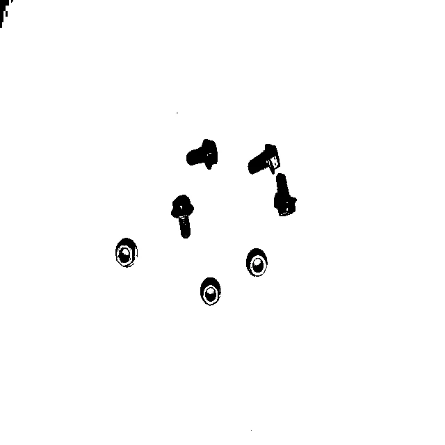
Yen selects a statistically preferred split; the application must verify that the split corresponds to the intended foreground.
3. Benchmarking
The 1995 paper evaluates the proposed criterion against other thresholding approaches and extends it to multiple levels. For a robot deployment, the relevant comparison is narrower and stricter: manual versus Otsu versus Yen on identical annotated camera frames. Report performance by contrast, foreground fraction, illumination, blur, texture, and target presence. Measure end-to-end latency through the hosted Skill rather than quoting only histogram-operation complexity.
4. Where to Go Next?
 Basic · 11 min read
What is Otsu Thresholding?
Otsu thresholding solves the problem of choosing one global intensity cutoff automatically from an image histogram. Learn its class-separation objective, assumptions, failure cases, and how to use it in the Telekinesis Agentic OS.
Read tutorial → Basic · 11 min read
What is Image Thresholding?
Image thresholding solves the problem of separating pixels with a known intensity cutoff. Learn the comparison modes, histogram reasoning, failure cases, evaluation metrics, and how to use global thresholding in the Telekinesis Agentic OS.
Read tutorial → Basic · 12 min read
What is Flood Fill Segmentation?
Flood fill segmentation solves the problem of extracting one connected, visually similar region from a known interior point. Learn seed-based region growing, tolerance and connectivity, failure modes, and how to use it in the Telekinesis Agentic OS.
Read tutorial → Basic · 13 min read
What is Contour Detection?
Contour detection solves the problem of recovering the exact outline of a foreground region by tracing an ordered boundary through a binary image. Learn how contour detection works, how contours are measured, and how to use it in the Telekinesis Agentic OS.
Read tutorial →5. References
- Yen, J.-C., Chang, F.-J., and Chang, S. “A New Criterion for Automatic Multilevel Thresholding”, IEEE Transactions on Image Processing, 1995.
- Otsu, N. “A Threshold Selection Method from Gray-Level Histograms”, IEEE Transactions on Systems, Man, and Cybernetics, 1979.
- Sezgin, M., and Sankur, B. “Survey over Image Thresholding Techniques and Quantitative Performance Evaluation”, Journal of Electronic Imaging, 2004.
- Telekinesis. “Segment Image Using Yen Threshold”, Cornea Skill documentation.