Imagine a camera above a backlit conveyor. The parts appear dark and the illuminated belt appears bright. If that contrast remains stable, the robot does not need a learned model to separate them. It needs one understandable rule: pixels on one side of an intensity cutoff belong to the parts; pixels on the other side belong to the background.
1. What is Image Thresholding?
Global image thresholding is a deterministic segmentation algorithm that compares every pixel with one fixed intensity cutoff. It solves foreground–background problems in which the two regions occupy reliably different intensity ranges.
“Global” means the same threshold is used everywhere. A pixel in the top-left corner and a pixel in the bottom-right corner face exactly the same decision. That simplicity makes the result fast, reproducible, and easy to audit. It also explains the main weakness: a shadow or lighting gradient can move otherwise identical surfaces to opposite sides of the threshold.
1.1 The Complete Thresholding Pipeline
One intensity cutoff → one label per pixel
A global threshold is predictable because the rule never changes, but that same rigidity makes it sensitive to illumination gradients.
Begin with a grayscale image in which every pixel stores one brightness value. The engineer chooses a cutoff, or threshold, that separates the values believed to belong to the foreground from those believed to belong to the background.
The algorithm then visits one pixel at a time. If its intensity falls on the selected side of the cutoff, it becomes foreground; otherwise it becomes background. Repeating that comparison across the image produces a binary mask that later code can count, measure, or use as a region of interest.
Nothing in this process understands objects. A bright reflection and a bright part receive the same label if their values cross the same threshold. Two equally dark pixels receive the same result even when they sit on opposite sides of the image. Thresholding works when intensity itself carries the answer and the lighting makes that answer separable.
The next sections first explain how a color image becomes a usable intensity and then show the exact decision made at each pixel.
1.2 From Color to One Intensity Value
Thresholding is easiest to understand for a grayscale image , where identifies a pixel and is its intensity. For an eight-bit image, intensities usually lie between 0 and 255.
If the source is RGB, the implementation must first reduce or otherwise interpret its channels. A common luma-like conversion is
, , and are gamma-encoded color channels, and is a brightness-like encoded value. The coefficients are not a universal law of cameras; they belong to a particular video/color convention. When precise behavior matters, convert to grayscale explicitly and inspect the actual values entering the threshold operation.
1.3 Binary Thresholding as a Decision Function
The basic binary rule is
is the global threshold, is the input intensity, and is the resulting label. Every pixel above becomes foreground. Binary inverse thresholding swaps the labels, which is useful when dark parts sit on a bright background.
The boundary convention—whether equality belongs above or below—must remain consistent. A one-level difference can affect many pixels when a large flat region lies exactly at the cutoff.
1.4 The Five Common Threshold Modes
The Telekinesis Skill exposes the familiar modes binary, binary_inv, trunc, tozero, and tozero_inv. Let be min_value, let be max_value, and let .
| Mode | Output rule | What it preserves |
|---|---|---|
binary | if , otherwise | Only the comparison result |
binary_inv | if , otherwise | Inverted comparison result |
trunc | if , otherwise | Dark values; clips bright values |
tozero | if , otherwise | Original bright intensities |
tozero_inv | if , otherwise | Original dark intensities |
Only the binary modes directly produce a two-valued image. The other modes are intensity transforms that can prepare an image for later processing. The parameter name max_value can therefore be misleading: it is the replacement value used by binary modes, not a second upper bound defining an accepted interval.
1.5 How to Choose the Threshold From a Histogram
An intensity histogram counts how many pixels have each gray level. If dark parts and a bright background form two distinct populations, the histogram often contains two peaks separated by a valley. Placing near that valley rejects many ambiguous pixels.
This is a calibration exercise. Capture representative images from the deployed camera, including normal brightness drift. Label target and background pixels, then inspect their distributions. A useful threshold leaves margin between the brightest valid dark pixel and the darkest valid bright pixel.
Do not tune from one attractive frame. Camera exposure, gain, white balance, surface reflectivity, and lamp aging all move the histogram. A threshold selected from only the nominal frame may fail during the first real production shift.
Interactive threshold
Move the cutoff and watch the decision change
Intensity histogram
Resulting one-dimensional mask
1.6 Why One Threshold Can Fail Across an Image
Suppose the left side of a conveyor receives more light than the right. The same gray part may produce intensity 80 on the left and 42 on the right. A threshold of 60 splits one physical material into foreground and background.
This failure is spatial, but a global threshold deliberately ignores position. Local or adaptive thresholding addresses it by calculating a neighborhood-dependent cutoff. Alternatively, the more reliable engineering fix may be diffuse illumination, locked exposure, or a light shield. Better optics and lighting often outperform extra software complexity.
1.7 Thresholding Has No Training Loss
Manual thresholding contains no learned parameters and uses no training dataset, so it has no loss function. The threshold is an engineering configuration value.
That does not remove the need for evaluation. For predicted foreground and annotated foreground , intersection over union is
contains correctly selected foreground pixels, and contains every pixel selected by either mask. Also report false-negative rate when missing a part is costly and false-positive rate when background pixels can trigger an unsafe pick.
1.8 From Pixel Labels to Robot Decisions
A binary mask becomes useful after spatial reasoning. Connected-component labeling groups neighboring foreground pixels into candidate parts. Area filtering rejects dust. Contours provide shape and perimeter. Moments provide centroids, and calibrated camera geometry maps those image coordinates into the robot workspace.
Thresholding itself supplies none of those guarantees. A bright reflection may form a valid foreground component. Two touching parts may merge. One part split by shadow may become two components. Validate the complete pipeline against the physical task.
1.9 When Should You Use a Manual Threshold?
| Situation | Recommendation |
|---|---|
| Fixed camera, stable backlight, known materials | Manual threshold is a strong baseline |
| Threshold changes between otherwise similar frames | Try Otsu or Yen and investigate exposure drift |
| Illumination varies across one frame | Use local/adaptive thresholding or improve lighting |
| Target is defined by color rather than intensity | Use RGB, HSV, LAB, or YCrCb segmentation |
| Target is selected from a known interior point | Flood fill may express the task better |
Manual thresholding is often the right industrial answer precisely because it is boring. When the workcell controls the image formation, a fixed rule is easy to validate and monitor. Automatic methods are valuable when the cutoff genuinely must adapt, not merely because they sound more sophisticated.
1.10 Calibrate a Threshold Without Guessing
Start with images, not a slider. Capture frames from the darkest and brightest valid operating conditions and annotate representative target and background regions. For every annotated pixel, record its grayscale intensity. You now have two empirical distributions rather than one visually chosen example.
If the distributions do not overlap, any threshold in the gap separates the sampled data. Choose a value with margin on both sides rather than placing it against one distribution. If they overlap, no single global threshold can classify every sampled pixel correctly. The overlap is evidence to improve lighting, restrict the region of interest, use another image feature, or accept a measured error rate.
Sweep candidate thresholds across the calibration set. For each value, calculate true positives, false positives, true negatives, and false negatives. Precision and recall are
counts correctly selected target pixels, counts background pixels incorrectly selected, and counts missed target pixels. Choose the operating point according to physical cost. A safety mask may prioritize recall; a pick proposal may prioritize precision to avoid grasping the background.
Freeze the chosen threshold with the camera configuration that produced it. Exposure, gain, gamma, white balance, bit depth, and grayscale conversion belong in the same versioned calibration record.
1.11 Noise, Blur, and Bit Depth Change the Boundary
Pixels close to the threshold can flip labels from frame to frame because of sensor noise. If , even a tiny variation changes the binary decision. A small denoising filter can stabilize flat regions, but blur also moves edges and can erase small defects. Evaluate preprocessing as part of the segmentation algorithm, not as a harmless cosmetic step.
Bit depth matters too. A threshold of 45 has different meaning in an eight-bit image, a normalized floating-point image, and a twelve-bit camera stream. Confirm the datatype and numeric range at the Skill boundary. Converting twelve-bit measurements to eight bits compresses 4096 possible values into 256 levels and can remove the intensity separation the inspection depended on.
Compression creates another source of variation. JPEG ringing around a sharp part boundary produces intensities not present on either physical surface. Lossless acquisition is preferable for metrology and fine defect segmentation.
1.12 Monitor the Rule After Deployment
A fixed threshold is easy to monitor because its expected behavior is stable. Track foreground fraction, connected-component count, mean foreground intensity, and mean background intensity. Slow drift can reveal lamp aging or lens contamination before segmentation fails completely. A sudden full-frame mask can indicate exposure or camera-setting failure.
Define explicit validity checks. For example, reject a result when the foreground covers less than 1% or more than 70% of the inspection region, when no component lies in the expected area range, or when the target centroid jumps farther than physically possible between synchronized frames. Thresholding creates the mask; operational monitoring decides whether that mask is credible enough for robot action.
2. How to Use Image Thresholding in the Telekinesis Agentic OS
Telekinesis provides global thresholding as the Cornea Skill segment_image_using_threshold. The code below loads the documented parts image, applies a binary threshold at intensity 45, and inspects the returned label map.
from telekinesis import cornea, datatypes

image = datatypes.Image.from_url(
    url="https://assets.telekinesis.ai/examples/v1/images/nuts_scattered.jpg"
).to_grayscale()

mask = cornea.segment_image_using_threshold(
    image=image,
    min_value=45,
    max_value=255,
    threshold_type="binary",
)

print(mask.shape)
print(mask.label_codes)
print(mask.number_of_labels)
The output shows the result of one fixed comparison. If foreground and background are reversed, use binary_inv; do not silently invert downstream assumptions without documenting which label represents the physical target.
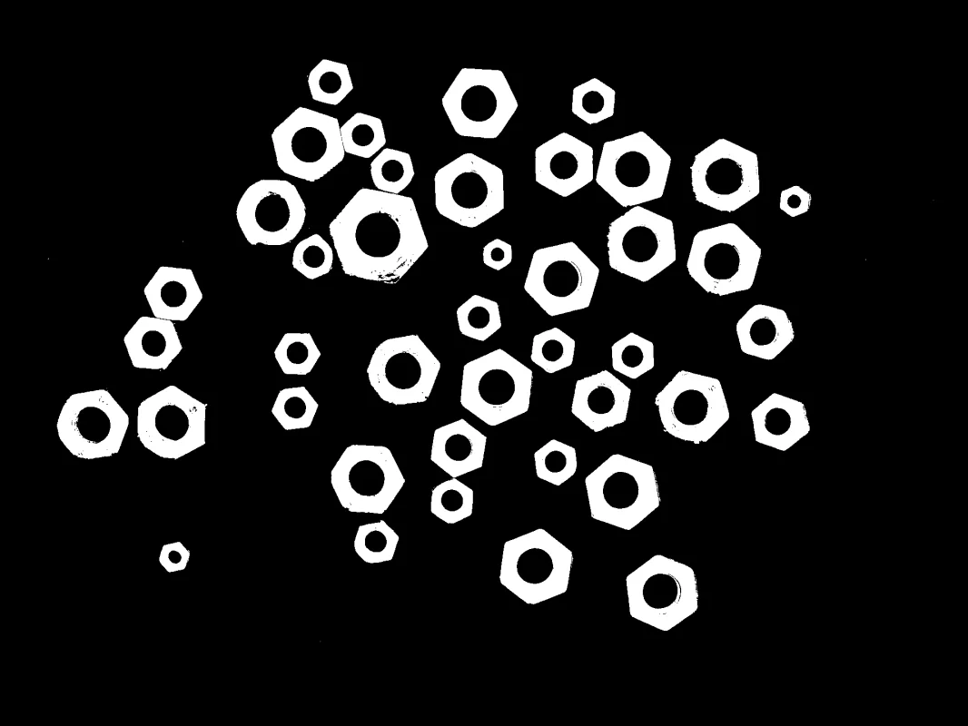
The mask is meaningful only under the intensity convention and lighting conditions used to choose the threshold.
3. Benchmarking
Benchmark the complete operating envelope, not only nominal accuracy. Sweep the threshold across a validation set and plot precision, recall, IoU, component count, and centroid error. Repeat under minimum and maximum permitted illumination, exposure, material finish, and background variation. Also record latency, although basic global thresholding is usually negligible compared with image transfer and service overhead.
4. Where to Go Next?
 Basic · 11 min read
What is Otsu Thresholding?
Otsu thresholding solves the problem of choosing one global intensity cutoff automatically from an image histogram. Learn its class-separation objective, assumptions, failure cases, and how to use it in the Telekinesis Agentic OS.
Read tutorial → Intermediate · 11 min read
What is Yen Thresholding?
Yen thresholding solves the problem of selecting one global intensity cutoff automatically with a probability-concentration criterion. Learn its histogram objective, difference from Otsu, limitations, and how to use it in the Telekinesis Agentic OS.
Read tutorial → Basic · 12 min read
What is Flood Fill Segmentation?
Flood fill segmentation solves the problem of extracting one connected, visually similar region from a known interior point. Learn seed-based region growing, tolerance and connectivity, failure modes, and how to use it in the Telekinesis Agentic OS.
Read tutorial → Basic · 14 min read
RGB vs HSV vs LAB vs YCrCb
RGB, HSV, LAB, and YCrCb describe the same pixel with different coordinates, making different segmentation problems easier. Learn what each channel means, how the transforms work, and which color space fits a robotics task.
Read tutorial →5. References
- Sezgin, M., and Sankur, B. “Survey over Image Thresholding Techniques and Quantitative Performance Evaluation”, Journal of Electronic Imaging, 2004.
- Otsu, N. “A Threshold Selection Method from Gray-Level Histograms”, IEEE Transactions on Systems, Man, and Cybernetics, 1979.
- Telekinesis. “Segment Image Using Threshold”, Cornea Skill documentation.