Classical Vision · Retina

What is Contour Detection?

Learn how a binary mask becomes an ordered outline with outer borders, holes, and hierarchy. Then use contour approximation and geometry to measure parts, inspect defects, and connect image pixels to robot coordinates.

Model: Border FollowingLevel: Basic

Imagine a robot inspecting a washer. A box around the washer shows where it is, but not whether its hole is missing or its edge is chipped. Contour detection follows the actual outline, giving the robot a shape it can measure.

1. What is Contour Detection?

Suppose a camera looks down at stamped washers on a bright conveyor. A detector can place a rectangle around each washer, which is enough to count them. But inspection asks more detailed questions: Is the outside edge round? Is the central hole present? Is a piece chipped from the rim?

To answer those questions, the system needs the shape itself. A contour is an ordered sequence of image coordinates that follows the boundary of a connected foreground region. Imagine tracing around the washer with a pencil without lifting the tip. The recorded path is its contour.

Because the boundary points remain in order, the robot can calculate area, perimeter, centroid, orientation, circularity, convexity, and local edge defects. A bounding box cannot preserve that information; it reduces the entire outline to four sides.

The contour algorithm does not know that the shape is a washer. It only knows which pixels are foreground and which are background. A shadow, oil stain, or glare can therefore create a perfectly valid—but meaningless—contour. This is why the story begins before contour detection: lighting, thresholding, and segmentation must first produce a useful binary image.

1.1 See the Full Contour Detection Pipeline

Image → ordered boundaries

ImageIntensity or colour

Binary maskForeground decision

Border followingRaster scan and boundary walk

Contour topologyOuter borders, holes, hierarchy

Ordered contoursBorders, holes, and hierarchy

Retrieval mode chooses topology; chain approximation chooses retained boundary detail.

Border following converts a binary mask into ordered boundaries, holes, and measurable topology. Adapted as an explanatory diagram fromSuzuki and Abe, border following.

Read the diagram from top to bottom. Image becomes a Binary mask. Border following walks around each foreground region, and Contour topology records outer borders, holes, and their hierarchy. The output is a collection of Ordered contours.

1.2 From an Image to an Ordered Boundary

The diagram begins at Image. Thresholding or segmentation converts that image into a Binary mask, where each pixel is classified as foreground or background. The quality of this mask determines which physical boundaries the algorithm can recover.

Border following scans across the mask until a pixel changes from background to foreground. That transition marks the beginning of a possible border. The algorithm then walks through neighbouring boundary pixels until it returns to the starting point.

This walk creates order. An edge detector may say that many pixels look like edges, but it does not necessarily say which pixels belong to one closed boundary. A contour groups them into a traversable path.

The influential method by Suzuki and Abe goes one step further. Its Contour topology stage records which boundaries surround others while the borders are traced. The final Ordered contours can therefore represent both the washer’s outside edge and the hole inside it.

1.3 How Contours Represent Holes Inside Objects

Think again about the washer. Its outside rim is an outer border because it encloses foreground material. The boundary around its opening is a hole border because it encloses background inside that material.

Suzuki and Abe’s first sequential algorithm assigns identifiers to borders during the image scan and records their parent–child relationships. The result preserves topology: not only which shapes exist, but which ones contain holes or nested regions.

The paper’s second algorithm follows only outermost borders. That lighter representation is enough when the goal is simply to count separate parts. The full hierarchy is needed when an internal hole carries engineering meaning, as it does for washers, rings, sockets, and drilled components.

1.4 How Many Boundary Points Should You Keep?

The raw contour may contain one point for almost every boundary pixel. Along a straight stamped edge, hundreds of those samples may describe the same line. Keeping them all preserves every small fluctuation, but it also increases memory, noise, and downstream computation.

Boundary approximation decides what to remember. A simple collinearity method removes redundant points along straight runs while retaining their endpoints. The Teh–Chin method uses local support and curvature to identify the dominant points of a digital curve.

This choice must follow the inspection requirement. If a two-pixel chip matters, aggressive simplification can erase the defect. If the robot only needs the overall orientation of a large plate, a compact polygon is easier to process than thousands of nearly identical points.

1.5 What Did Suzuki and Abe Add?

The important innovation is the combination of geometry and hierarchy. Suzuki and Abe do not merely trace lines. Their algorithms recover outer borders, hole borders, and the relationships between them during one sequential scan. An engineer can therefore ask both “what is the shape?” and “what is inside what?”

1.6 How to Measure a Contour

Once the contour has been extracted and simplified appropriately, it becomes measurable geometry. For vertices $(x_i, y_i)$ ordered around a closed polygon, the signed shoelace area is

A = \frac{1}{2}\sum_{i=0}^{n-1}(x_i y_{i+1} - x_{i+1}y_i), \qquad (x_n,y_n)=(x_0,y_0).

The sign reveals traversal direction; the magnitude estimates enclosed pixel area. The perimeter is the distance travelled while walking once around the boundary:

P = \sum_{i=0}^{n-1}\sqrt{(x_{i+1}-x_i)^2+(y_{i+1}-y_i)^2}.

Area and perimeter together produce the scale-independent compactness measure called circularity:

C = \frac{4\pi |A|}{P^2}.

An ideal mathematical circle has $C=1$ ; elongated or irregular shapes have smaller values. Real circles also score below one because pixels form stair-stepped boundaries and image noise changes the perimeter. Image moments similarly provide the centroid, $c_x=m_{10}/m_{00}$ and $c_y=m_{01}/m_{00}$ .

At this point the robot can compare the measured washer with its specification. But the measurements are still in pixels. A contour centroid becomes a robot pick point only after camera calibration and a depth or plane model connect image coordinates to physical coordinates. Shape extraction provides the geometry; calibration places that geometry in the robot’s world.

1.7 When Should You Use Contours?

Representation	Preserves	Best question
Edge map	Local intensity transitions	“Where does appearance change?”
Contour	Ordered region boundary	“What is this outline’s geometry?”
Bounding box	Coarse rectangular extent	“Where is the object approximately?”
Segmentation mask	Every classified pixel	“Which pixels belong to the object?”

The representations answer different questions, so they often work together. A learned detector can first locate the washer, segmentation can separate it from the conveyor, and a contour can perform the precise geometric inspection. Use contours when the outline carries the answer; use semantic models when appearance or identity matters more than boundary shape.

2. How to Use Contour Detection in the Telekinesis Agentic OS

Telekinesis provides contour extraction as the Retina Skill detect_contours. The code below loads a grayscale image, selects the retrieval and approximation modes, filters contours by area, and prints each returned boundary’s shape.

from telekinesis import datatypes, retina

image = datatypes.Image.from_url(
    url=(
        "https://assets.telekinesis.ai/examples/v1/images/"
        "nuts_scattered_filtered_gaussian.png"
    )
).to_grayscale()

contours = retina.detect_contours(
    image=image,
    retrieval_mode="retrieve_list",
    approx_method="chain_approximate_simple",
    min_area=200,
    max_area=100_000,
)

print(f"Detected {len(contours.points)} contours")
for index, points in enumerate(contours.points):
    print(index, points.shape)  # (K_i, 2), with (x, y) coordinates

The output makes the variable-length geometry visible. Check that the traced boundaries follow the physical parts—not shadows, glare, or texture—before computing measurements from them.

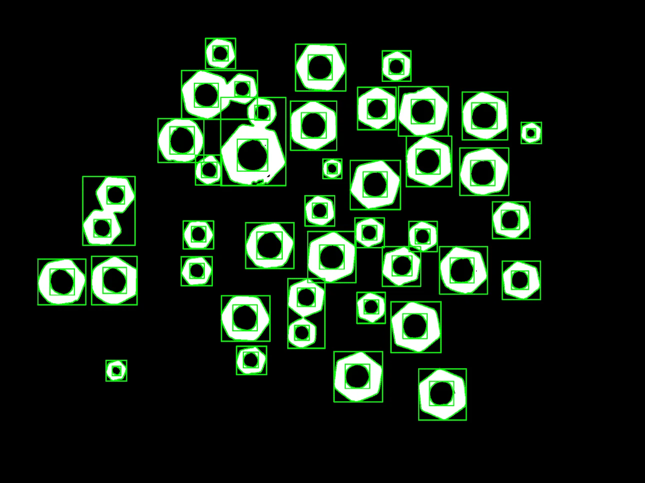
Contours returned by the Retina Skill

The output follows the visible part boundaries. Whether an outline is useful still depends on the quality and meaning of the foreground image.

3. Benchmarking

3.1 Evidence Reported in the Original Research

The 1985 Suzuki–Abe paper predates COCO-style benchmark tables. It establishes algorithmic behavior and demonstrates component counting, shrinking, and topology extraction rather than reporting a portable AP or FPS score. A faithful summary is therefore qualitative:

Paper evaluation dimension	Reported capability
Input	Digitized binary images
Output	Outer borders, hole borders, and surroundness relations
Algorithm style	Sequential border following during raster scan
Demonstrated uses	Component counting, shrinking, topological analysis
Important limitation	Result quality inherits the binary foreground definition

For a robot workcell, benchmark boundary precision/recall against annotated masks, centroid and area error against metrology, false accept/reject rate, and end-to-end latency at the deployed resolution.

4. Where to Go Next?

If the parts are circular and their radius range is known, continue with the Classic Hough Transform. For semantic objects in changing scenes, compare YOLOX and RF-DETR.

5. References

Suzuki, S., and Abe, K. “Topological Structural Analysis of Digitized Binary Images by Border Following”, Computer Vision, Graphics, and Image Processing, 1985.
Teh, C.-H., and Chin, R. T. “On the Detection of Dominant Points on Digital Curves”, IEEE Transactions on Pattern Analysis and Machine Intelligence, 1989.
Ramer, U. “An Iterative Procedure for the Polygonal Approximation of Plane Curves”, Computer Graphics and Image Processing, 1972.
Douglas, D. H., and Peucker, T. K. “Algorithms for the Reduction of the Number of Points Required to Represent a Digitized Line or Its Caricature”, Cartographica, 1973.