Imagine a robot approaching a workbench with two cameras mounted a few centimetres apart. A bolt appears slightly farther to the left in one image than in the other. That small shift is not a nuisance: together with the camera geometry, it reveals how far the bolt is from the robot.
Card image credit: architecture overview from the Fast-FoundationStereo project page, by Bowen Wen, Shaurya Dewan, and Stan Birchfield, NVIDIA.
1. What is Fast-FoundationStereo?
Fast-FoundationStereo is a real-time neural stereo-matching model that estimates disparity from a rectified pair of images and generalizes to scenes not used for task-specific fine-tuning. Disparity is the horizontal displacement of the same scene point between the left and right images. Once disparity is known, calibrated stereo geometry converts it into metric depth.
This distinction is the first useful mental model. The network does not directly discover metres from pixels. It solves a correspondence problem: for each useful point in the left image, where is the matching point in the right image? The focal length and physical distance between the cameras then give that correspondence a metric scale.
Fast-FoundationStereo builds on FoundationStereo, which was designed for strong zero-shot stereo matching but was expensive to run. The newer model keeps the same broad pipeline—feature extraction, cost filtering, and iterative disparity refinement—while accelerating each part through knowledge distillation, neural architecture search, and structured pruning.
1.1 The Complete Path From Two Images to Depth
Rectified stereo pair → disparity → metric depth
The network predicts disparity; calibrated camera geometry—not the neural network alone—turns that disparity into meters.
The pipeline starts with two cameras viewing the same scene from slightly different horizontal positions. Before the model sees the images, calibration and rectification place matching scene points on the same image row. This turns a difficult search across the whole second image into a search left or right along one line.
Both images then pass through the same feature network. The network replaces raw color patches with learned descriptions that are easier to compare across the two views. For each location in the left image, a cost volume records how well it matches candidate locations in the right image at different horizontal shifts.
Some matches are obvious; others are ambiguous because a surface is textureless, repeated, reflective, or partly hidden. The model uses surrounding image context to filter those possibilities, chooses an initial shift for every pixel, and improves that disparity estimate through several refinement steps.
Only then does camera geometry convert disparity into metric depth. Large left–right shifts usually indicate nearby points; small shifts indicate distant points. Keeping learned matching separate from this final geometric conversion makes the assumptions clear, so we begin the deep dive with rectification and disparity.
1.2 Stereo Geometry Turns Image Shift Into Distance
Two cameras see the same 3D point from different horizontal positions. In raw images, lens distortion and camera rotation can place the corresponding pixels almost anywhere. Stereo rectification warps both images so that corresponding points lie on the same image row. Matching can then search horizontally rather than across an entire image.
Let a scene point appear at horizontal coordinate in the left image and in the right image. Its disparity is
Here, is disparity in pixels, while and are horizontal pixel coordinates in the rectified images. For a conventional stereo arrangement, nearby points move farther between views and therefore have larger disparity.
Depth follows from similar triangles:
is depth along the camera’s forward axis in metres, is the horizontal focal length expressed in pixels, is the stereo baseline in metres, and is disparity in pixels. Because the pixel units cancel, the result inherits the baseline’s unit.
Suppose pixels, metres, and pixels. The estimated depth is metres. If the measured baseline is wrong by ten percent, the resulting depth scale is wrong by ten percent too. No learned model can repair incorrect calibration supplied after matching.
The inverse relationship also explains the range limit. At long distances, disparity becomes very small. A one-pixel disparity error then creates a large depth error. Stereo is strongest where the baseline, focal length, image resolution, and working distance produce measurable displacement.
Interactive stereo geometry
Disparity turns horizontal image shift into depth
Large disparity means the corresponding pixels are far apart and the point is close. Small disparity means the point is far away, where one-pixel errors matter much more.
1.3 The Backbone Extracts Features From Both Views
Comparing raw RGB pixels is fragile. A surface can look slightly different between cameras because of exposure, reflections, occlusion, or sensor noise. Fast-FoundationStereo first turns each image into a pyramid of learned feature maps. Fine maps preserve edges and small objects; coarser maps carry wider context.
FoundationStereo obtained rich priors from a hybrid backbone that combined stereo features with a large monocular vision foundation model. That helped generalization but cost too much for real-time use. Fast-FoundationStereo distils those hybrid teacher features into one efficient student backbone.
For feature level , the distillation objective can be written as
is the feature-distillation loss; is the student’s feature map at pyramid level ; is the frozen teacher feature at the same level; and sums squared element-wise differences. A projection aligns channel dimensions when the teacher and student widths differ.
The student is therefore not merely trained to reproduce the teacher’s final disparity. It is taught to construct similar intermediate evidence at several spatial scales.
1.4 A Cost Volume Stores Possible Correspondences
The backbone has described both images, but it has not yet selected matches. The next stage creates a cost volume. For every left-image location, it compares the left feature with right-image features at a range of candidate disparities.
Conceptually, a matching score can be pictured as
is the evidence for disparity at left-image pixel ; and are left and right feature vectors; and is a learned or correlation-based similarity operation. Rectification is visible in the equation: the row remains fixed while only the horizontal coordinate changes.
The max_disp setting limits the tested values of . A larger range covers closer objects or wider baselines but increases computation and memory. If the true disparity falls outside the range, the correct match is unavailable regardless of how good the later network is.
A raw cost volume remains ambiguous. A blank wall offers many nearly identical matches. Repetitive shelves create several plausible displacements. Occluded pixels may have no counterpart at all. This is why stereo networks need cost filtering rather than independently choosing the best number at every pixel.
1.5 Cost Filtering Uses Context to Resolve Ambiguity
Cost filtering lets neighbouring evidence and long-range scene structure influence each match. FoundationStereo used a powerful combination of 3D processing and transformer reasoning over the cost volume. Fast-FoundationStereo seeks cheaper blocks that preserve as much of that behaviour as possible.
Instead of searching complete networks from scratch, the paper divides the filtering network into local blocks. Candidate replacements for each block are trained to mimic the corresponding frozen teacher block:
is candidate for block position ; is the teacher block; is the teacher feature entering that position; and is the squared feature-reconstruction loss. For the last block, which predicts initial disparity rather than an intermediate feature, the paper uses smooth supervision against ground truth.
Each candidate is then inserted into the full teacher pipeline and measured for both error and runtime. Integer linear programming selects one candidate per position under a latency budget. This blockwise approach makes an otherwise enormous combinatorial search practical and produces several speed–accuracy variants rather than one universal network.
1.6 A Pruned ConvGRU Refines Disparity Iteratively
The filtered cost volume supplies an initial disparity, but boundaries and difficult regions still need correction. A convolutional gated recurrent unit, or ConvGRU, repeatedly examines the current disparity, matching evidence, and hidden state. Each iteration predicts an update rather than restarting the map.
If denotes disparity after iteration , the process can be summarized as
is the previous estimate and is the correction predicted at iteration . The Telekinesis valid_iters parameter controls how many of these refinement steps run.
Recurrent networks contain linked channel dependencies: pruning one output can invalidate a later recurrent input. The paper constructs a dependency graph, ranks parameters using a first-order Taylor approximation, prunes unimportant structure consistently, and retrains the reduced refinement module.
Its retraining loss is
is the number of refinement iterations; is predicted disparity after iteration ; is ground-truth or trusted pseudo-label disparity; gives later iterations greater weight; is the number of refinement layers; and are student and teacher features at layer ; and balances output accuracy against feature distillation.
This equation teaches the two goals clearly. The first term makes every recurrent estimate geometrically accurate. The second keeps the pruned network’s internal computation near the stronger teacher.
1.7 What the Model Was Trained On
Fast-FoundationStereo uses the mixed stereo training data inherited from FoundationStereo and adds 1.4 million pseudo-labeled in-the-wild stereo pairs. FoundationStereo’s own dataset contains roughly one million high-fidelity synthetic pairs designed to include difficult materials, low-texture regions, reflections, and occlusion.
For the additional real imagery, the authors do not blindly trust one teacher prediction. Their pipeline compares stereo estimates with monocular depth through surface-normal consistency, corrects scale where appropriate, and masks unreliable sky regions. Temporal subsampling removes near-duplicate video frames. The surviving pseudo-labels add real-world visual variety while feature distillation transfers the teacher’s internal priors.
“Zero-shot” therefore means the released model is intended to work on new stereo scenes without fine-tuning for each deployment domain. It does not mean the model was trained without data, nor that every new camera, material, or weather condition will work equally well.
1.8 Where Stereo Depth Fails
Occlusion: a point visible to one camera may be hidden from the other, so no valid correspondence exists.
Weak texture: a blank surface provides few distinctive features. Context can help, but the match remains less observable.
Repetition: identical slats, shelves, or holes support several plausible disparities.
Reflections and transparency: the two cameras may observe different reflected content rather than one stable surface point.
Calibration or synchronization error: rectification assumes a rigid, known stereo pair and near-simultaneous capture. Moving objects can violate row alignment when exposures occur at different times.
Disparity range: very close objects may exceed max_disp; very distant objects may have too little disparity for reliable metric depth.
The model can generalize visual matching better than classical block matching, but it does not remove the geometry’s observability limits.
1.9 Engineering Trade-offs for a Robot
Increasing max_disp expands the near working range but grows the cost volume. Increasing valid_iters adds recurrent computation, but this distilled model is tuned around the default eight iterations; more iterations are not guaranteed to improve it. A wider physical baseline increases disparity and improves depth resolution at distance, yet also creates larger occluded regions and makes matching close objects harder. A longer focal length similarly increases disparity but narrows field of view.
Benchmark the complete sensing chain. Record capture synchronization, rectification, service latency, invalid-depth rate, and depth error by distance and material. For manipulation, report error in the final 3D point or pose rather than judging only whether the depth visualization looks smooth.
2. How to Use Fast-FoundationStereo in the Telekinesis Agentic OS
Telekinesis provides Fast-FoundationStereo as the Vitreous Skill estimate_depth_using_fast_foundation_stereo. The code below creates a simple rectified stereo pair with 20 pixels of disparity, supplies the left camera intrinsics and a 5 cm baseline, and requests metric depth.
import numpy as np

from telekinesis import datatypes, vitreous

height, width = 480, 640
disparity_px = 20
baseline = 0.05

rng = np.random.default_rng(0)
texture = rng.integers(
    0, 255, (height, width + disparity_px, 3), dtype=np.uint8
)
left_image = datatypes.Image(texture[:, :width])
right_image = datatypes.Image(
    texture[:, disparity_px : disparity_px + width]
)

camera_calibration = datatypes.CameraCalibration(
    width=width,
    height=height,
    distortion_model="plumb_bob",
    distortion_parameters=[0.0, 0.0, 0.0, 0.0, 0.0],
    intrinsic_matrix=[
        600.0, 0.0, 320.0,
        0.0, 600.0, 240.0,
        0.0, 0.0, 1.0,
    ],
)

depth_image = vitreous.estimate_depth_using_fast_foundation_stereo(
    left_image=left_image,
    right_image=right_image,
    camera_calibration=camera_calibration,
    baseline=baseline,
    valid_iters=8,
    max_disp=192,
)

valid_depth = depth_image.depth[depth_image.depth > 0]
print("Depth shape:", depth_image.depth.shape)
print("Median valid depth:", np.median(valid_depth))
The synthetic shift corresponds to metres. Real inputs must already be rectified, share the same resolution, and come from a calibrated, synchronized stereo rig. The returned DepthImage uses metres; zero marks pixels without valid depth, and its color plane is aligned to the left image.
3. Benchmarking
3.1 Zero-Shot Results Reported in the Paper
The Fast-FoundationStereo paper evaluates all methods without fine-tuning on the target datasets. The full paper table reports bad-pixel rates at several thresholds; this compact version uses BP-2 for Middlebury, BP-1 for ETH3D, and D1 for KITTI. Lower is better. Runtime is measured on Middlebury-Q with an NVIDIA RTX 3090.
| Method | Middlebury-H BP-2 ↓ | Middlebury-Q BP-2 ↓ | ETH3D BP-1 ↓ | KITTI 2012 D1 ↓ | KITTI 2015 D1 ↓ | Runtime ↓ |
|---|---|---|---|---|---|---|
| StereoAnywhere | 4.75 | 3.25 | 1.43 | 2.81 | 3.52 | 427 ms |
| MonSter | 4.24 | 3.19 | 0.99 | 2.84 | 3.41 | 336 ms |
| FoundationStereo | 1.10 | 1.30 | 0.50 | 2.30 | 2.80 | 496 ms |
| RT-IGEV, same training mixture | 7.82 | 5.59 | 5.05 | 3.25 | 4.00 | 45 ms |
| LightStereo-L, same training mixture | 12.55 | 7.70 | 16.34 | 3.73 | 4.51 | 30 ms |
| Fast-FoundationStereo | 2.20 | 2.12 | 1.22 | 2.35 | 3.25 | 49 ms / 21 ms TensorRT |
The comparison shows the intended compromise: FoundationStereo remains more accurate, but Fast-FoundationStereo cuts the paper’s RTX 3090 runtime by roughly tenfold while staying much closer to it than other real-time models.
3.2 Non-Lambertian Surfaces
Booster-Q includes reflective and transparent surfaces that violate the simple stereo assumption that corresponding pixels look alike.
| Method | BP-2 ↓ | BP-4 ↓ | BP-6 ↓ | BP-8 ↓ | EPE ↓ | Real-time |
|---|---|---|---|---|---|---|
| StereoAnywhere | 9.01 | 5.40 | 4.12 | 3.34 | 1.21 | No |
| FoundationStereo | 5.18 | 4.07 | 2.91 | 2.59 | 1.13 | No |
| RT-IGEV, same training mixture | 18.19 | 13.39 | 11.37 | 10.16 | 4.20 | Yes |
| Fast-FoundationStereo | 6.61 | 4.62 | 3.91 | 3.49 | 1.54 | Yes |
3.3 Efficiency and Ablations
| Method | RTX 3090 | RTX 4090 | A100 | Parameters | MACs |
|---|---|---|---|---|---|
| FoundationStereo | 496 ms | 295 ms | 308 ms | 374.5M | 5,413.9G |
| Fast-FoundationStereo | 49 ms | 30 ms | 41 ms | 14.6M | 309.9G |
The feature-distillation ablation shows why the paper uses mean-squared error (MSE):
| Distillation strategy | Middlebury-H BP-2 ↓ | ETH3D BP-1 ↓ | KITTI 2012 D1 ↓ | KITTI 2015 D1 ↓ |
|---|---|---|---|---|
| None | 2.87 | 2.11 | 2.67 | 4.32 |
| Cosine similarity | 2.29 | 1.19 | 2.39 | 3.31 |
| MSE | 2.20 | 1.22 | 2.35 | 3.25 |
The 1.4-million-pair pseudo-labeled dataset also improves the final model from 2.53 to 2.20 BP-2 on Middlebury-H, 1.31 to 1.22 BP-1 on ETH3D, 2.44 to 2.35 D1 on KITTI 2012, and 3.48 to 3.25 D1 on KITTI 2015.
3.4 What to Measure on a Robot
The standard disparity metric is end-point error:
is the set of evaluated pixels; is predicted disparity at pixel ; is reference disparity; and is the number of evaluated pixels. Also report the fraction exceeding a task-relevant disparity or depth error.
For robotics, stratify results by distance, material, texture, occlusion, and motion. Measure metric depth error, invalid pixels, boundary error, latency percentiles, and the accuracy of downstream 3D positions. Paper measurements do not include your capture, rectification, network transport, or target accelerator.
4. Where to Go Next
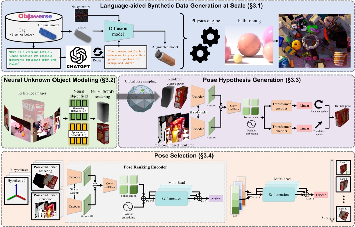 Advanced · 16 min read
What is FoundationPose?
FoundationPose solves the problem of locating a previously unseen rigid object in 3D when its shape is known. Learn how pose hypotheses are rendered, refined, ranked, and tracked, which losses train the model, and how to use it in the Telekinesis Agentic OS.
Read tutorial →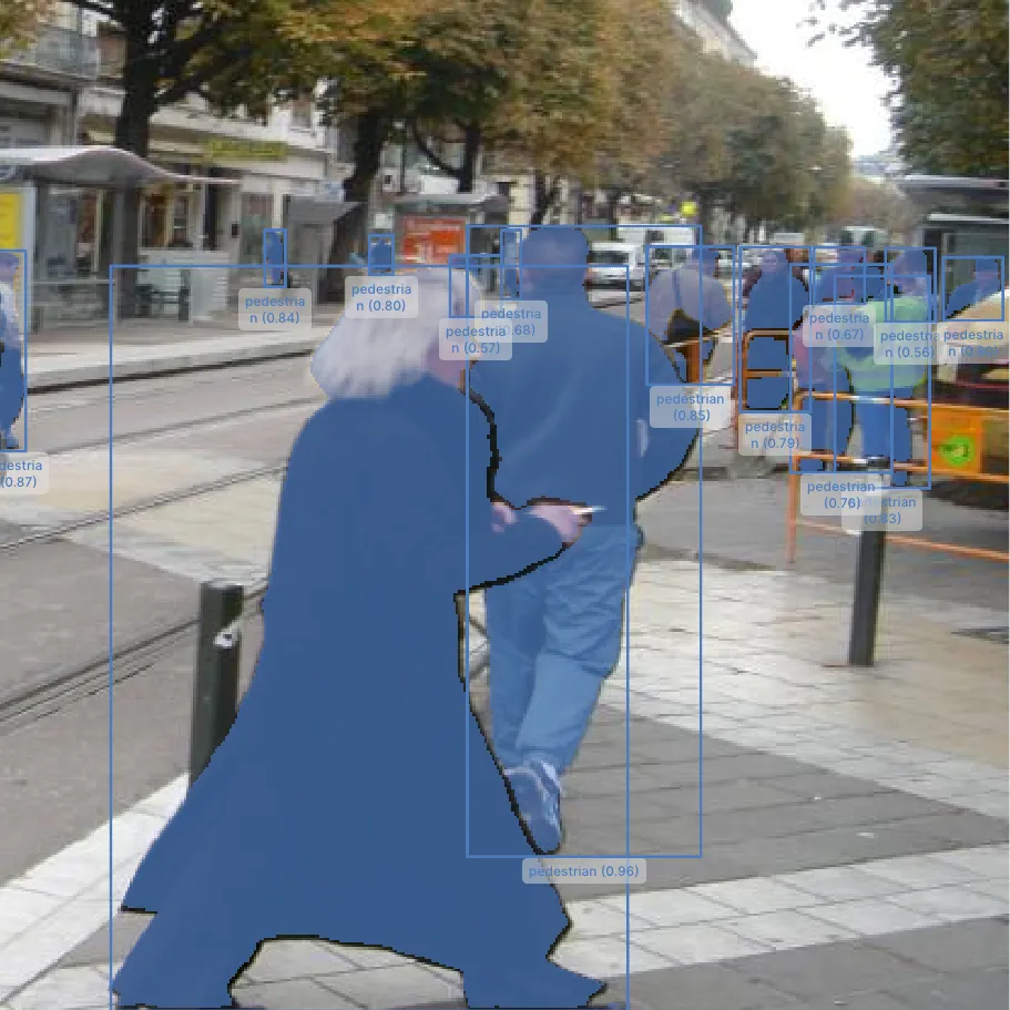 Intermediate · 13 min read
What is SAM 3?
SAM 3 solves the problem of finding and precisely segmenting every image region that matches a text concept or visual prompt. Learn its promptable concept segmentation architecture, training losses, data engine, and how to use it in the Telekinesis Agentic OS.
Read tutorial →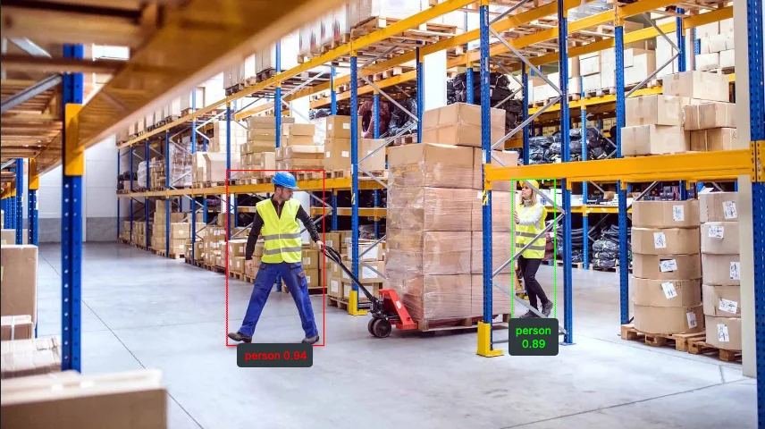 Intermediate · 17 min read
What is RF-DETR?
RF-DETR solves the problem of detecting known objects accurately within a tight latency budget by using a real-time detection transformer. Learn the architecture of RF-DETR, the loss functions it was trained with, and how to use it in the Telekinesis Agentic OS.
Read tutorial →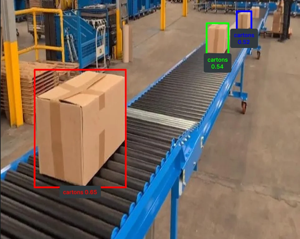 Intermediate · 16 min read
What is Grounding DINO?
Grounding DINO solves the problem of locating objects described in ordinary language by using an open-vocabulary object detection model. Learn the architecture of Grounding DINO, the loss functions it was trained with, and how to use it in the Telekinesis Agentic OS.
Read tutorial →5. References
- Wen, B., Dewan, S., and Birchfield, S. “Fast-FoundationStereo: Real-Time Zero-Shot Stereo Matching”, CVPR 2026.
- Wen, B. et al. “FoundationStereo: Zero-Shot Stereo Matching”, CVPR 2025.
- Scharstein, D. and Szeliski, R. “A Taxonomy and Evaluation of Dense Two-Frame Stereo Correspondence Algorithms”, International Journal of Computer Vision, 2002.
- Telekinesis. “Estimate Depth Using Fast-FoundationStereo”, Vitreous Skill documentation.