Imagine a cobot picking long metal profiles from a tray. Object segmentation has already produced one point cloud per profile, but the robot still needs a compact answer to three questions: Where is this part? Which way is it pointing? How much space does it occupy? The centroid, principal axes, and 3D bounding boxes answer those geometric questions without needing a trained object model.
Input
Output
1. What Are Principal Axes and 3D Bounding Boxes?
Principal axes and bounding boxes summarize the position, orientation, and extent of a 3D point set. They are useful after a point cloud has been filtered and separated into individual objects, when passing every raw point to planning would be unnecessarily expensive.
The centroid is the average position of the points. The principal axes describe the directions in which the cloud spreads most, second most, and least. An axis-aligned bounding box (AABB) is the smallest box aligned with the current coordinate frame’s X, Y, and Z axes that contains every point. An oriented bounding box (OBB) is allowed to rotate, so it can follow the object’s own geometry more tightly.
These quantities are related, but they are not interchangeable. AABB answers “what world-aligned region contains this cloud?” OBB answers “what rotated box compactly encloses it?” Principal axes answer “along which directions are these samples distributed?” For a robot, choosing the correct summary is more important than choosing the mathematically fanciest one.
1.1 From Object Points to a Geometric Summary
3D object samples → orientation and extent
Axes describe directions of spread, not semantic front, left, or up; symmetry and outliers can make that orientation ambiguous.
The workflow starts with one isolated object. If the input still contains a tabletop, a neighboring object, or flying depth points, those measurements become part of the geometry and can change every result downstream.
First compute the center. Centering turns absolute camera coordinates into offsets around the object, so the following calculation measures shape rather than location. Next summarize how those offsets vary together. PCA does this with a covariance matrix; an OBB method instead searches for axes that describe a compact enclosing box.
The recovered axes form a candidate local frame for the object. Projecting points into that frame reveals their length, width, and height. The final result is a small geometric description—a center, directions, and dimensions—that a planner can use for cropping, collision approximation, approach selection, or grasp orientation.
1.2 The Centroid Separates Location From Shape
For a cloud containing positions , the centroid is
is the number of points; is point ; and is their mean 3D position. The centered vector describes point relative to this center.
The centroid is easy to compute, but it is not necessarily the physical center of mass. Depth cameras sample visible surfaces rather than material volume. If only the front of a part is visible, the point centroid shifts toward that visible side. Uneven density and outliers also move it. Treat it as the center of the measured samples unless the sensing process justifies a stronger interpretation.
1.3 PCA Finds Directions of Maximum Spread
Principal component analysis begins with the covariance matrix
is a symmetric matrix. Its diagonal entries describe variation along X, Y, and Z; its off-diagonal entries describe how two coordinates vary together. We then solve
is eigenvector , and is its eigenvalue. Sort them so . The first principal axis points along the largest spread; captures the next-largest perpendicular spread; and captures the least. For a flat plate, often approximates the surface normal. For a long bar, follows its length.
The fraction
is the proportion of total positional variance along axis . is dimensionless. A long thin object has one dominant value; a roughly spherical cloud has three similar values and therefore no strongly preferred orientation.
1.4 Why Principal Directions Can Flip or Become Ambiguous
An eigenvector has an unavoidable sign ambiguity. If is an eigenvector, represents the same axis. A principal axis can therefore point in either direction between runs without the underlying line changing. Geometry alone cannot decide which end of a symmetric profile is its “front.”
There is a second ambiguity when eigenvalues are equal or nearly equal. A cylindrical can may have one stable long axis, but any two perpendicular directions around that axis describe almost the same spread. A cube can make all three directions unstable. Small noise may rotate the returned frame dramatically even though the object barely moved.
For stable robot orientation, add a convention: point one axis toward the camera, align the least-varying axis with gravity, use color or a key feature to identify the front, and enforce a right-handed frame. Principal axes propose a geometric frame; these rules make it temporally and semantically consistent.
1.5 AABB: Fast Bounds in the Current Coordinate Frame
An axis-aligned box is defined directly by coordinate-wise extrema:
and are opposite corners. The box dimensions are , and its volume is , where , , and are its extents.
AABB is fast, deterministic, and always aligned with the frame used by the rest of the system. This makes it excellent for broad-phase collision checks, workspace indexing, and quickly cropping a known world region. Its weakness is rotation: a long diagonal part creates a large box containing substantial empty space.
1.6 OBB: Let the Box Follow the Object
An oriented box introduces a center , an orthonormal rotation matrix , and local dimensions . A world point lies inside when its local coordinates
satisfy , , and . Here, is the world point, is the box center, contains the box axes as columns, and is the same point expressed in the box frame.
An OBB can be derived from candidate object axes and then tightened, or searched to reduce enclosing volume. Telekinesis exposes minimize_bbox_volume for a tighter result and use_robust_fitting when noisy data requires a less brittle fit. Both options trade additional computation for a better geometric summary.
Interactive 3D bounds
Rotate the part and compare world-aligned and object-aligned boxes
The interactive view shows why neither box is universally better. AABB stays meaningful in the world frame as the part rotates, but its size changes. OBB follows the part and usually stays compact, but its orientation can be unstable for symmetric geometry. Pick based on the downstream question.
1.7 Outliers and Partial Views Change the Answer
Extrema make bounding boxes especially sensitive to distant points. One stray measurement can stretch an AABB or OBB far beyond the part. Covariance spreads the influence across all points, but a sufficiently distant outlier contributes a large squared offset and can rotate PCA axes.
Clean the cloud before summarizing it. Crop the workspace, remove statistical or radius outliers, and cluster separate objects. Then test partial views deliberately. An industrial arm may see only the upper surface of a part in one pose and a side surface in another. If those visible samples produce different axes, the principal frame is not a reliable substitute for full 6D model-based pose estimation.
1.8 Which Representation Should You Use?
| Representation | Best question | Strength | Important limitation |
|---|---|---|---|
| Centroid | “Where is the average measured position?” | Minimal, fast location cue | Not necessarily center of mass |
| PCA axes | “How is this cloud distributed?” | Direct shape-orientation summary | Sensitive to outliers and symmetry |
| AABB | “What world-aligned region contains it?” | Fast and stable in the world frame | Loose for rotated objects |
| OBB | “What rotated box encloses it compactly?” | Tight extent and useful orientation cue | More compute; orientation may be ambiguous |
| FoundationPose / registration | “What is the object’s model-relative 6D pose?” | Semantic/model-aware orientation | Requires a model, initialization, or more compute |
Use the simplest representation that preserves the information required by the task. AABB may be sufficient for AMR obstacle indexing. OBB may give an industrial arm a useful approach direction for a long profile. A keyed aerospace component whose rotation matters around every axis needs a model-aware pose method.
2. How to Use Principal Axes and 3D Boxes in the Telekinesis Agentic OS
The three Vitreous Skills can operate on the same isolated cloud:
from telekinesis import datatypes, vitreous

point_cloud = datatypes.PointCloud.from_url(
    url=(
        "https://assets.telekinesis.ai/examples/v1/point_clouds/"
        "zivid_large_pcb_inspection_cropped_preprocessed.ply"
    ),
    use_cache=True,
)

principal_axes = vitreous.estimate_principal_axes(
    point_cloud=point_cloud,
    method="obb",  # Use "pca" for the covariance-based method.
)

aabb = vitreous.calculate_axis_aligned_bounding_box(
    point_cloud=point_cloud,
)

obb = vitreous.calculate_oriented_bounding_box(
    point_cloud=point_cloud,
    minimize_bbox_volume=True,
    use_robust_fitting=True,
)

print("AABB dimensions:", aabb.dimensions, "volume:", aabb.volume)
print("OBB dimensions:", obb.dimensions, "volume:", obb.volume)
print("principal axes:", principal_axes)
The pca method is fast for clean data. The obb method uses the oriented-box axes and is intended to be more robust on noisy clouds. Do not compare the two only on one visually clean scan; compare orientation repeatability across the full camera and object operating range.
3. How to Evaluate a Geometric Summary
There is no single benchmark score for centroids, axes, and boxes because they answer different questions. Evaluate each output against its intended robot use:
| Metric | Definition | Why it matters |
|---|---|---|
| Center error | Euclidean distance to a reference center | Measures localization drift |
| Axis angular error | Smallest angle between estimated and reference axes | Measures orientation quality while respecting sign ambiguity |
| Box IoU | Intersection volume divided by union volume | Measures agreement of 3D occupied regions |
| Volume ratio | Estimated volume divided by reference volume | Reveals loose or outlier-stretched boxes |
| Repeatability | Variation across repeated scans of a static part | Exposes sensor and symmetry instability |
| Task success | Pick, insertion, or collision-check success | Verifies that the abstraction is useful downstream |
Separate errors caused by the summarizer from errors caused by segmentation. Run the geometry first on clean reference clouds, then on realistic clustered sensor data. That tells you whether to improve the box method or the upstream perception pipeline.
4. Where to Go Next
 Intermediate · 10 min read
What is DBSCAN Point-Cloud Clustering?
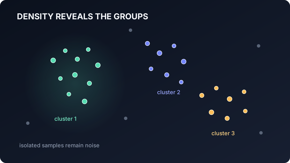
DBSCAN separates a point cloud into dense connected groups without requiring the number of clusters in advance. Learn core, border, and noise points, density reachability, parameter tuning, computational trade-offs, and how to use DBSCAN in the Telekinesis Agentic OS.
Read tutorial →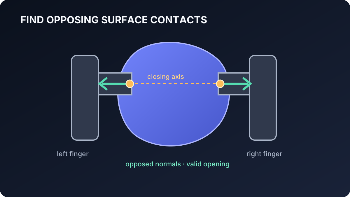 Advanced · 11 min read
What is Antipodal Grasp Sampling?
Antipodal grasp sampling proposes parallel-jaw grasps by finding opposing contacts on an object surface. Learn contact normals, friction intuition, grasp-frame construction, candidate scoring and validation, and how to generate grasps in the Telekinesis Agentic OS.
Read tutorial →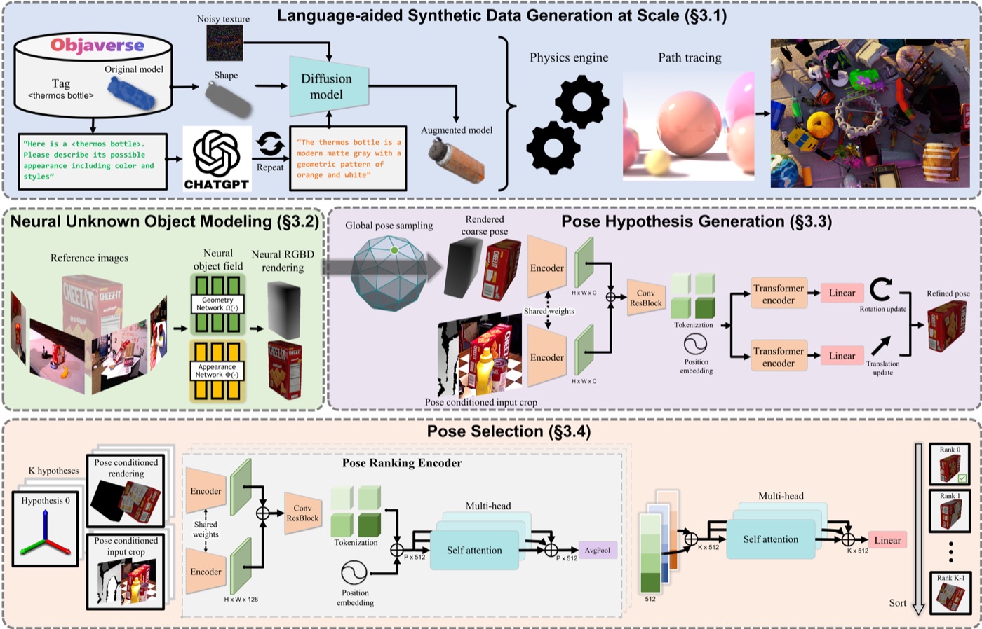 Advanced · 16 min read
What is FoundationPose?
FoundationPose solves the problem of locating a previously unseen rigid object in 3D when its shape is known. Learn how pose hypotheses are rendered, refined, ranked, and tracked, which losses train the model, and how to use it in the Telekinesis Agentic OS.
Read tutorial →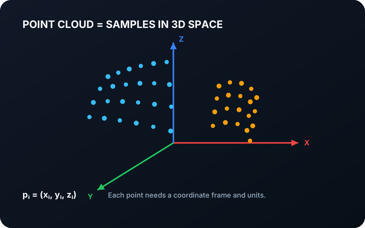 Basic · 4 min read
What is a Point Cloud?
A point cloud is a collection of sampled positions in three-dimensional space. Learn how points represent visible geometry, why coordinate frames matter, and how depth images become spatial data for robots.
Read tutorial →5. References
- Pearson, K. “On Lines and Planes of Closest Fit to Systems of Points in Space”, Philosophical Magazine, 1901.
- Telekinesis. “Estimate Principal Axes”, Vitreous Skill documentation.
- Telekinesis. “Calculate Axis-Aligned Bounding Box”, Vitreous Skill documentation.
- Telekinesis. “Calculate Oriented Bounding Box”, Vitreous Skill documentation.