Imagine a drone scanning an industrial structure or an arm inspecting a cast part. The depth sensor returns thousands of points sampled from visible surfaces, but those points are disconnected. A collision checker cannot tell which gaps are empty and which simply lie between samples. Mesh reconstruction adds that missing connectivity by inferring a surface and expressing it as triangles.
Input
Output
1. How Do Point Clouds Become Meshes?
Mesh reconstruction solves the problem of turning disconnected 3D samples into a connected surface. A point cloud tells us where measurements exist. A triangle mesh additionally states which vertices are neighbors and which triangular faces fill the space between them.
That extra structure enables operations that are awkward on raw points: rendering solid surfaces, testing ray intersections, estimating enclosed volume, constructing simplified collision geometry, and exchanging models with CAD or simulation tools. But the surface is not directly measured everywhere. It is inferred. Every reconstruction method therefore embeds assumptions about smoothness, closure, missing views, and object shape.
This tutorial compares two useful extremes. A convex hull wraps the cloud in the smallest convex shell. It is fast, closed, and conservative, but it fills every dent and opening. Poisson reconstruction uses oriented surface normals to fit a smooth implicit surface, so it can represent concavity and more detail. It needs better input and can also invent plausible surfaces where data is missing.
1.1 The Complete Reconstruction Pipeline
Discrete 3D samples → connected surface
A mesh is an inference between samples: the algorithm’s assumptions decide how gaps, concavities, and missing views are filled.
Start by asking what the output is for. Collision avoidance may prefer a simple conservative shell. Inspection or digital-twin visualization may need recessed surfaces and curved detail. The requirement determines the surface assumption.
Next prepare the input. Convex hull needs point positions. Poisson reconstruction additionally needs normals whose directions are reasonably consistent. Downsampling can reduce redundant samples, while outlier removal prevents isolated measurements from creating spikes or expanding the result.
The reconstruction algorithm then builds an internal representation. Convex hull reasons directly about enclosing facets. Poisson builds an adaptive spatial field and solves for an implicit inside/outside function. Finally, the inferred boundary is extracted as connected vertices and triangle indices. The mesh must still be checked for size, artifacts, unwanted closure, and suitability for the downstream robot task.
1.2 What a Triangle Mesh Stores
Let the mesh contain vertices
and triangular faces
is the 3D position of vertex ; is the number of vertices; each tuple references three vertex indices; and is the number of faces. The indexed representation reuses vertices between neighboring triangles rather than storing three independent points for every face.
A mesh is watertight when its faces form a closed boundary with no open edges. Watertightness is useful for volume and inside/outside tests, but it is not the same as truth. An algorithm can close the open top of a scanned container and produce a perfectly watertight but physically incorrect model.
1.3 Convex Hull: Wrap the Cloud With a Tight Convex Shell
A set is convex when the straight line segment between any two points in the set remains inside it. The convex hull of point set is the smallest convex set containing every point. Equivalently,
is the input point set; are non-negative weights that sum to one; and contains every convex combination of the input points. The boundary facets of this set form the convex-hull mesh.
Picture stretching plastic film tightly around the cloud. The film touches extreme points and spans directly across gaps. That behavior makes the hull robust to missing interior samples and useful as conservative collision geometry. It also makes concavity impossible: a U-shaped bracket becomes closer to a solid block, and a mug handle’s opening may disappear.
The joggle_inputs option slightly perturbs degenerate input so the hull computation can handle cases such as nearly coplanar points. It can rescue a numerical problem, but it does not add genuine 3D information. A truly planar cloud does not define a meaningful enclosed 3D volume.
1.4 Why Poisson Reconstruction Needs Oriented Normals
Poisson reconstruction starts from a different observation. A surface normal tells us which way the local surface faces. If normals are consistently oriented outward, they resemble samples of the gradient of an object’s indicator function.
Define an ideal indicator that is approximately 1 inside the object and 0 outside. Its change is concentrated around the boundary. Poisson reconstruction builds a vector field from the point normals, then solves
is the unknown scalar indicator field; is the Laplacian operator; is divergence; and is the vector field formed from oriented samples. Another view is that the method seeks a field whose gradient matches the normal field:
is the reconstructed spatial domain, is the gradient of the indicator field, and the integral accumulates disagreement across space. Taking the variational condition of this least-squares objective yields the Poisson equation above.
The final surface is an isosurface , where is a selected field value. An isosurface extraction step converts that continuous boundary into triangles.
This explains the normal requirement. Positions say where the surface was sampled; oriented normals say how the inside/outside field should change there. Randomly flipped normals create contradictory evidence. Noisy normals create ripples, bulges, or incorrect closure.
1.5 The Octree Controls Where Detail Can Exist
Representing a dense 3D field on one uniform grid is expensive because doubling resolution along X, Y, and Z creates roughly eight times as many cells. Poisson reconstruction uses an octree, which recursively divides occupied regions into eight smaller cubes.
octree_depth controls the finest allowed subdivision. Each extra level approximately halves the smallest cell width, so it can preserve finer features but increases memory, computation, and sensitivity to noise. Higher depth cannot recover detail that was never sampled; it can only give the solver more capacity to follow the available evidence.
octree_width offers another way to specify target resolution, while scale_factor expands the reconstruction domain around the samples. Too little scale can clip the solution near the boundary. Excess scale spends resolution on empty space and may change how the surface closes.
Interactive surface reconstruction
Change the method and see what happens to concave geometry
The visual isolates the central trade-off. The convex hull deliberately bridges the recess. Poisson can follow it because its implicit field is not restricted to convex shapes. Neither output is automatically correct: the first may be too conservative, while the second depends on sufficient oriented evidence.
1.6 How Missing Views Affect the Result
A single depth camera rarely observes an object’s entire surface. The back and underside may contain no points. Reconstruction must still decide what happens there.
Convex hull closes missing areas with planar facets. This tends to overestimate occupied space, which can be acceptable for safety margins but poor for fit checking. Poisson prefers a globally smooth closed solution. It may form a smooth cap across an unseen opening or extend a surface beyond the measured region. The result can look convincing precisely because the algorithm produces continuity.
For accurate object geometry, register multiple views before reconstruction. Record camera poses, remove moving objects, and verify that normal orientation remains consistent after transforms. If the task only needs a collision proxy, a deliberately simplified hull may be more honest than a visually detailed hallucination.
1.7 Preparing a Cloud for Reconstruction
A robust workflow usually performs these steps:
- Crop the workspace. Remove walls, fixtures, and distant geometry that do not belong to the object.
- Separate the target. Use masks, clustering, plane removal, or model-based pose to isolate one surface.
- Remove outliers. Isolated points can create hull spikes or Poisson artifacts.
- Balance density. Voxel downsampling prevents one close camera view from dominating the reconstruction.
- Estimate and orient normals. Select a neighborhood that follows real surface curvature without following sensor noise.
- Reconstruct and trim. Remove low-confidence or unwanted regions when the method exposes suitable confidence information.
- Validate in task space. Check clearance, dimensions, and collisions using known references.
The order matters. Reconstructing first and cleaning later converts measurement errors into connected surface geometry, which is often harder to recognize and remove.
1.8 Choosing Between Convex Hull and Poisson
| Requirement | Convex hull | Poisson reconstruction |
|---|---|---|
| Input | 3D positions | 3D positions plus oriented normals |
| Output shape | Always convex | Smooth and potentially concave |
| Missing regions | Bridged conservatively | Smoothly inferred and closed |
| Fine detail | Not represented inside the hull | Controlled by samples, normals, and octree resolution |
| Typical cost | Lower | Higher |
| Good robotics use | Broad collision proxy, coarse occupied volume | Surface visualization, detailed geometry, watertight model |
| Main risk | Overfills openings and recesses | Creates plausible surfaces unsupported by measurements |
If the object is already approximately convex and speed matters, use the hull. If concavity matters and normals are trustworthy, use Poisson. For thin sheets, open surfaces, sharp CAD-like edges, or topology that must remain open, neither default may be suitable without additional processing or a different reconstruction family.
2. How to Reconstruct Meshes in the Telekinesis Agentic OS
The following example produces both representations from official sample clouds. Poisson input must already contain normals.
from telekinesis import datatypes, vitreous

oriented_cloud = datatypes.PointCloud.from_url(
    url=(
        "https://assets.telekinesis.ai/examples/v1/point_clouds/"
        "industrial_part_7_normals.ply"
    ),
    use_cache=True,
)

poisson_mesh = vitreous.reconstruct_mesh_using_poisson(
    point_cloud=oriented_cloud,
    octree_depth=8,
    octree_width=0,
    scale_factor=1.05,
)

hull_mesh = vitreous.reconstruct_mesh_using_convex_hull(
    point_cloud=oriented_cloud,
    joggle_inputs=False,
)

print("Poisson triangles:", len(poisson_mesh.triangle_indices))
print("Hull triangles:", len(hull_mesh.triangle_indices))
Compare the two meshes against the same cloud in a 3D viewer. Look especially at holes, recesses, thin walls, unseen backs, and isolated points. Triangle count alone says nothing about geometric truth.
3. How to Benchmark a Reconstructed Mesh
A visually smooth mesh can still be dimensionally wrong. Use reference geometry when available and report several complementary measures:
| Metric | What it measures | Limitation |
|---|---|---|
| Point-to-surface distance | Distance from measured or reference samples to the mesh | One direction can miss extra invented surface |
| Chamfer distance | Average nearest distance in both directions | Averages can hide local worst cases |
| Hausdorff distance | Largest nearest-surface deviation | Very sensitive to a single outlier |
| Normal consistency | Agreement of local surface orientation | Requires trustworthy reference normals |
| Completeness | Fraction of reference surface within a tolerance | Depends on reference coverage |
| Watertightness / manifold checks | Topological validity for downstream geometry | Valid topology does not imply accurate shape |
| Triangle count and runtime | Deployment cost | More triangles do not guarantee more truth |
For collision use, compare false-free-space and false-occupied-space volumes. For inspection, measure dimensional error at critical features. For grasp planning, run collision and contact checks on the reconstructed mesh, then measure real execution success. Choose octree_depth from this evidence rather than from visual smoothness alone.
4. Where to Go Next
 Basic · 10 min read
What is Voxel Downsampling?
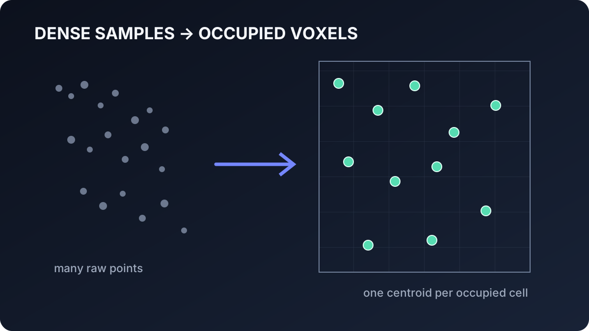
Voxel downsampling reduces a dense point cloud by replacing samples in each occupied 3D cell with their centroid. Learn how voxel indexing and averaging work, how voxel size trades geometric detail for speed, and how to use the filter in the Telekinesis Agentic OS.
Read tutorial →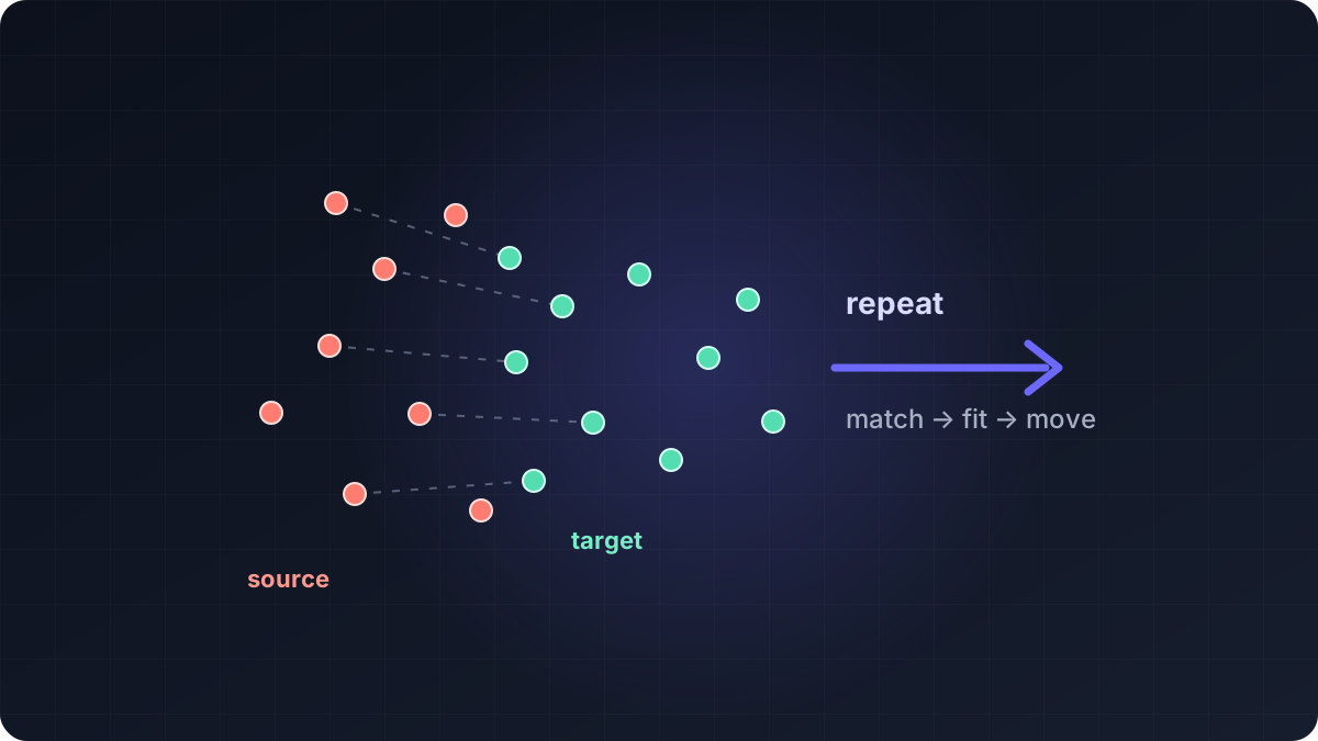 Advanced · 17 min read
What is Iterative Closest Point (ICP)?
Point-cloud registration solves the problem of placing two 3D scans in the same coordinate frame, and ICP does this by repeatedly matching nearby points and fitting a rigid transform. Learn point-to-point and point-to-plane ICP, Fast Global Registration, their mathematics and failure modes, and how to build a coarse-to-fine registration pipeline in the Telekinesis Agentic OS.
Read tutorial →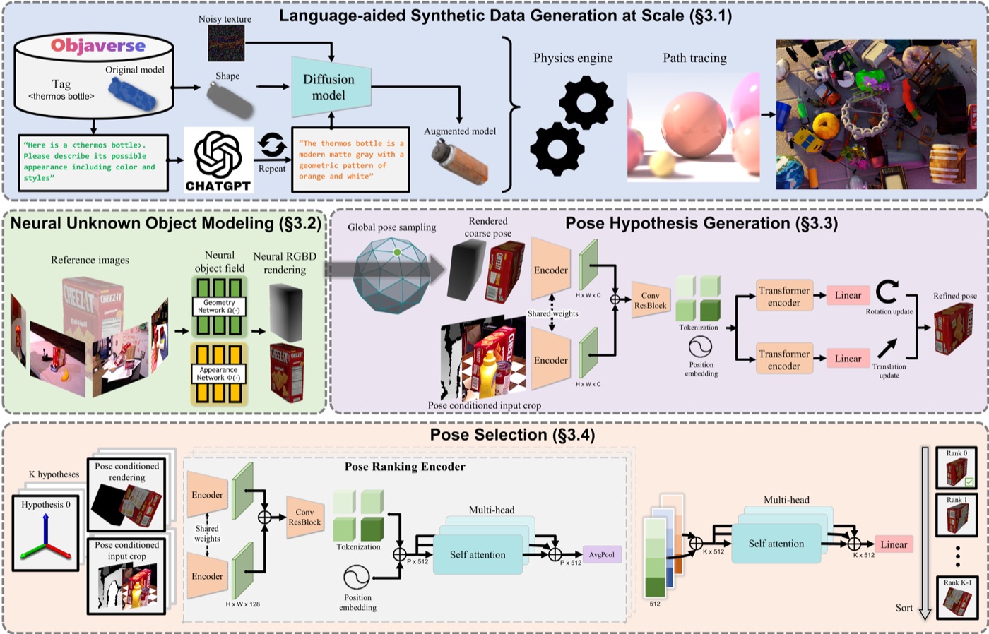 Advanced · 16 min read
What is FoundationPose?
FoundationPose solves the problem of locating a previously unseen rigid object in 3D when its shape is known. Learn how pose hypotheses are rendered, refined, ranked, and tracked, which losses train the model, and how to use it in the Telekinesis Agentic OS.
Read tutorial →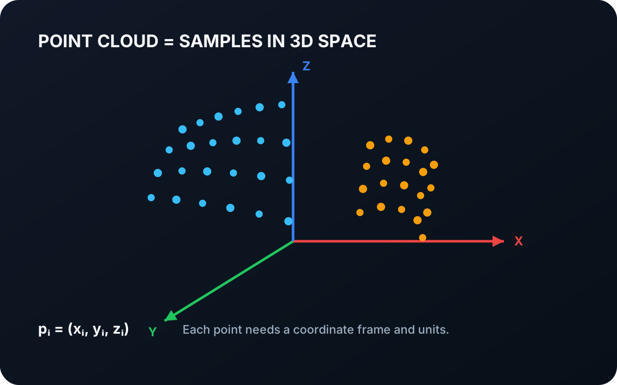 Basic · 4 min read
What is a Point Cloud?
A point cloud is a collection of sampled positions in three-dimensional space. Learn how points represent visible geometry, why coordinate frames matter, and how depth images become spatial data for robots.
Read tutorial →5. References
- Kazhdan, M., Bolitho, M., and Hoppe, H. “Poisson Surface Reconstruction”, Eurographics Symposium on Geometry Processing, 2006.
- Barber, C. B., Dobkin, D. P., and Huhdanpaa, H. “The Quickhull Algorithm for Convex Hulls”, ACM Transactions on Mathematical Software, 1996.
- Telekinesis. “Reconstruct Mesh Using Poisson”, Vitreous Skill documentation.
- Telekinesis. “Reconstruct Mesh Using Convex Hull”, Vitreous Skill documentation.