Imagine an industrial arm inspecting a machined plate. It does not need to know that the metal has brightness value 142; it needs the exact rim of a drilled hole, the outside of the part, and the line of a possible crack. Edge detection converts sharp brightness changes into numerical responses that later geometry can measure.
1. What is Edge Detection?
Edge detection measures how quickly image intensity changes across neighboring pixels. This tutorial builds a directional-gradient mental model, explains Sobel, Scharr, and Laplacian filters, and shows how to compute their responses with Pupil.
An edge is not automatically an object boundary. Texture, shadows, highlights, printed labels, and sensor noise can all create sharp intensity changes. Edge detection answers “where does appearance change?” A later stage must decide what that change means.
1.1 The Edge Detection Pipeline
Intensity changes → directional gradients
Sobel and Scharr estimate the first derivative and preserve direction; the Laplacian estimates a direction-free second derivative.
Picture a camera image from a pick-and-place industrial arm: a bright aluminum part lies on a dark conveyor. Along a row of pixels inside either surface, brightness changes very little. At the physical boundary, the values jump sharply. Edge detection measures this jump without needing to know what aluminum or conveyor means.
The diagram measures change in two directions. One filter moves conceptually from left to right and records how quickly intensity changes along the X axis. Another does the same from top to bottom along Y. Keeping both measurements matters because a boundary can face any direction in the image.
The names can feel backward at first. A vertical line is crossed by moving horizontally, so it produces a strong X-direction response. A horizontal line is crossed by moving vertically, so it produces a strong Y response. Combining those two responses gives the edge strength, while their relative sizes reveal the edge direction.
The output is evidence about rapid image change, not an object outline. Texture, shadows, printed labels, and sensor noise can all create edges. Later stages must decide which responses connect into useful boundaries.
1.2 A Derivative on a Pixel Grid
Suppose a drone captures the image of a wing-panel seam. Brightness changes slowly on the flat panel and rapidly at the seam. A derivative measures that rate of change, turning the visual idea of a boundary into a number. Before choosing Sobel or Scharr, we need to understand what the horizontal and vertical derivative images represent.
For a continuous intensity function , the image gradient is
is image intensity at coordinate , while and are its horizontal and vertical derivatives. Digital images contain samples rather than a continuous function, so kernels approximate these derivatives from nearby pixels.
The gradient magnitude and orientation are commonly computed as
is edge strength and is the direction of maximum intensity increase. The visible boundary runs perpendicular to that direction.
1.3 Sobel: Differentiate and Smooth Together
A warehouse AMR searching for shelf uprights needs stable vertical boundaries even when the image contains sensor noise and printed carton texture. A two-pixel subtraction reacts strongly to every tiny fluctuation because it uses almost no context. Sobel uses a neighborhood to estimate change while performing a small amount of smoothing in the perpendicular direction.
The Sobel kernels are
estimates and estimates . The central row or column receives more weight, which introduces a small amount of smoothing in the direction perpendicular to the derivative. This makes Sobel less sensitive to isolated noise than the simplest two-pixel difference.
Pupil exposes derivative orders as dx and dy. Use dx=1, dy=0 for the first X derivative, or dx=0, dy=1 for Y. Asking for both at once is not the same as computing two separate gradient images and combining their magnitude; it requests a mixed derivative configuration. For a conventional magnitude, compute X and Y separately and combine downstream.
Interactive mechanism
Choose a derivative and see which boundaries respond
Intensity image
Selected response
1.4 Why Signed Output Matters
Computing the derivative is only useful if its output type can represent the result. This matters because direction has a sign: crossing a boundary from dark to bright should not produce the same number as crossing it from bright to dark.
One derivative is positive and the other negative. If the output is stored directly in an unsigned 8-bit image, negative values are clipped to zero and half the directional information disappears.
Use a signed or floating output_format, such as 64bit, when the sign matters or when gradients will be combined mathematically. Convert to an absolute display image only for visualization. This is a data-type decision, not cosmetic formatting.
The scale parameter multiplies the derivative and delta adds an offset. These parameters can help with representation, but they do not recover information lost by clipping or saturation.
1.5 Scharr: A Better Small Directional Kernel
A humanoid can approach the same furniture edge from many angles. Ideally, that edge should produce a similar response as its orientation changes. Sobel’s smallest kernel is slightly biased by the pixel grid; Scharr offers a more rotationally balanced approximation.
Scharr changes the coefficients to improve rotational symmetry at that fixed size. It is useful when a compact kernel and accurate directional response matter.
Sobel remains useful because its kernel size is configurable. Larger kernels measure change over a wider neighborhood, which suppresses fine noise but also changes the scale of edges being emphasized. Scharr is fixed at .
1.6 Laplacian: Measure the Second Derivative
An industrial arm looking for fine scratches may not know their orientation in advance. Sobel and Scharr measure directional first derivatives. The Laplacian instead measures how the rate of brightness change changes and combines both axes, making it useful when the response should not prefer horizontal or vertical structure.
The Laplacian is
is the Laplacian response. Around a blurred step edge, the response changes sign and crosses zero near the boundary. Because a second derivative amplifies high-frequency noise strongly, smoothing before the Laplacian is often essential.
Use Sobel or Scharr when direction is useful. Use the Laplacian when an isotropic second-derivative response is the desired feature. None of these operators performs hysteresis, edge linking, or semantic grouping by itself.
1.7 From Gradient Response to a Usable Boundary
Derivative operators return measurement images, not finished object outlines. Before they can support contour tracing or geometry, we need to turn broad, noisy responses into a smaller set of credible boundary pixels.
A raw gradient image is usually dense. A practical pipeline may smooth first, compute derivatives, form a magnitude, suppress weak responses, and then connect or trace the surviving pixels. The threshold must be tested against both real boundaries and the strongest nuisance texture.
The order matters. Smoothing after differentiation does not undo noisy derivative peaks in the same way as smoothing the image first. Record the complete pipeline, including color conversion, filter, derivative, output depth, magnitude rule, and threshold.
1.8 Follow One Edge Through the Mathematics
The operators are easier to connect when we follow one physical boundary rather than comparing isolated equations. Imagine sampling brightness along a horizontal line that crosses from a dark surface to a bright one.
An ideal step changes instantly. A real lens and pixel grid blur it into a ramp. The first derivative is small on either flat surface, rises through the ramp, and reaches its largest magnitude near the center of the transition. That peak is the edge estimate.
The second derivative describes how the first derivative changes. It is positive on one side of the first-derivative peak, negative on the other, and crosses zero near the edge center. This connects the operators: Sobel and Scharr look for a first-derivative peak, while a Laplacian pipeline can look for second-derivative zero crossings.
Noise contains rapid changes, so differentiation amplifies it. A simple finite difference illustrates the problem:
If either sample contains independent noise, their difference contains both errors. A second derivative combines still more alternating contributions. This is why derivative scale and prior smoothing are inseparable design choices.
1.9 Edge Scale Determines What Counts as a Boundary
Once we know how a single edge creates a response, the next decision is which size of change should count. Kernel size and prior smoothing define the spatial scale of the detector, so they also define which details disappear.
A narrow derivative kernel responds to fine texture, printed marks, and sharp noise. A wider Sobel kernel or stronger Gaussian prefilter responds to broader transitions and ignores some small variation. Neither is universally more accurate: they answer questions at different spatial scales.
Suppose a cable boundary spans three pixels because it is slightly out of focus. A very small operator may produce several irregular responses across the ramp. Smoothing at approximately that scale can yield one stable peak. But if two cables are separated by only four pixels, the same smoothing may merge their transitions.
Build a scale test containing the narrowest gap and smallest boundary required by the task. Evaluate position error and separation, not just edge-map cleanliness.
1.10 Gradient Direction Supports More Than Visualization
Edge strength tells us whether something changes; gradient direction tells us how it changes. Keeping that second quantity can make later geometry more selective instead of treating every strong response equally.
The angle points in the direction of increasing intensity. It can reject irrelevant edges: an AMR searching for vertical shelf uprights may retain responses with near-horizontal gradients. It can also support contour following, line fitting, Hough voting, and feature descriptors.
Direction becomes unreliable when magnitude is close to zero because tiny noise determines the ratio between and . Apply an edge-strength gate before interpreting orientation. Remember that reversing contrast rotates the signed gradient by 180 degrees even though the visible boundary has the same undirected orientation.
1.11 Thresholding and Linking Turn Responses Into Edges
The last step is to decide which measured responses form the edge map consumed downstream. This is not merely cosmetic binarization: it determines whether faint boundaries remain connected and whether nuisance texture survives.
A derivative produces a continuous response, not a final binary boundary. One threshold removes weak values but creates a difficult trade-off: a high threshold breaks faint real edges, while a low threshold admits texture.
A common strategy uses two thresholds. Strong responses start accepted edges; weaker responses survive only when connected to strong ones. Non-maximum suppression can thin a broad gradient ridge by keeping local maxima along the gradient direction. These ideas explain why a complete edge detector is more than a Sobel call.
Pupil’s Sobel, Scharr, and Laplacian Skills deliberately expose the derivative evidence. That is useful when the next stage needs signed gradients or custom logic rather than a prepackaged binary edge map.
1.12 Common Failure Modes in Robot Images
The preceding mechanisms tell us what an edge detector measures, which makes its failures easier to diagnose. Many strong image changes are real measurements but do not correspond to the physical object boundary the robot needs.
- Specular highlights: a shiny part produces strong internal edges unrelated to geometry.
- Cast shadows: the boundary belongs to illumination rather than the object.
- Motion blur: the transition spreads, reducing peak magnitude and shifting localization.
- Texture: labels, machining marks, and floor patterns create many legitimate intensity changes.
- Clipping: saturated regions lose internal gradients entirely.
- Borders: padding rules can create artificial responses at the image boundary.
The remedy depends on cause. Diffuse lighting addresses highlights; synchronized exposure addresses motion; a region of interest rejects irrelevant texture; border configuration prevents synthetic image-boundary edges. Threshold tuning alone cannot solve every failure.
2. How to Compute Sobel Gradients in the Telekinesis Agentic OS
To retain the information described above, compute the horizontal and vertical derivatives separately and keep a signed output format. The example does exactly that, leaving magnitude, orientation, and thresholding available for the downstream task.
from telekinesis import datatypes, pupil

image = datatypes.Image.from_url(
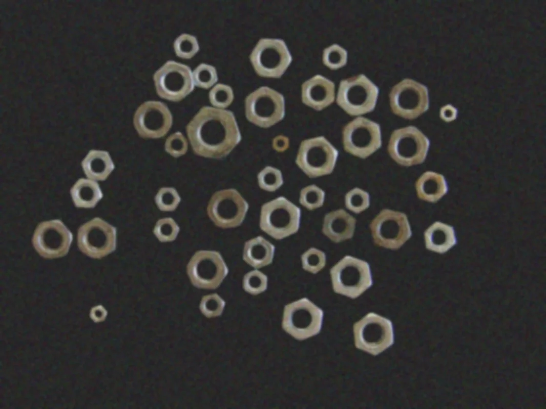
    url="https://assets.telekinesis.ai/examples/v1/images/nuts.jpg"
).to_grayscale()

gradient_x = pupil.filter_image_using_sobel(
    image=image,
    output_format="64bit",
    dx=1,
    dy=0,
    kernel_size=3,
    scale=1.0,
    delta=0.0,
    border_type="default",
)

gradient_y = pupil.filter_image_using_sobel(
    image=image,
    output_format="64bit",
    dx=0,
    dy=1,
    kernel_size=3,
    scale=1.0,
    delta=0.0,
    border_type="default",
)

print(gradient_x.shape, gradient_y.shape)
Keep the signed responses for computation. If the final task is measuring a contour, validate the recovered boundary position rather than judging only whether the gradient image looks crisp.
3. How to Evaluate an Edge Pipeline
Edge evaluation must reflect how the response will be used. With annotated boundaries, report precision and recall within a small pixel tolerance because two valid edge traces may differ by one pixel. For metrology, measure the resulting line, center, diameter, or pose error. Also test low contrast, textured surfaces, motion blur, exposure changes, and image borders.
Kernel size and preprocessing must remain fixed during comparison. A larger Sobel kernel may look calmer but shift or broaden the response. The correct setting is the one that makes the downstream geometry repeatable on the deployed camera.
4. Where to Go Next
 Basic · 14 min read
What is Image Filtering?
Image filtering changes each pixel using nearby pixels so that useful structure becomes easier to measure. Learn how box, Gaussian, median, and bilateral filters work, what their parameters mean, and how to choose one in the Telekinesis Agentic OS.
Read tutorial → Basic · 13 min read
What is Contour Detection?
Contour detection solves the problem of recovering the exact outline of a foreground region by tracing an ordered boundary through a binary image. Learn how contour detection works, how contours are measured, and how to use it in the Telekinesis Agentic OS.
Read tutorial →5. References
- Telekinesis. “Filter Image Using Sobel”, Pupil Skill documentation.
- Scharr, H. “Optimal Operators in Digital Image Processing”, 2000.
- Marr, D., and Hildreth, E. “Theory of Edge Detection”, 1980.